Download

1 / 59
590 likes | 721 Vues
Regional Impacts of State jobs in Denmark The General Interregional Quantity Model. by Bjarne Madsen. Bjarne Madsen. Statslige arbejdspladser – definition & statistik Lidt polemik Konsekvenser af statslige arbejdspladser - mængdemodel 2 gange 2 gange 2 princippet – SAM-K and LINE

E N D
Regional Impacts of State jobs in DenmarkThe General Interregional Quantity Model by Bjarne Madsen Bjarne Madsen
Statslige arbejdspladser – definition & statistik Lidt polemik Konsekvenser af statslige arbejdspladser - mængdemodel 2 gange 2 gange 2 princippet – SAM-K and LINE Modellering af konsekvenser af statslige arbejdspladser Disposition
Gymnasier fra amtskommuner til staten Sociale institutioner fra amtskommunerne til kommunerne Fordeling af jobs på ejerkode - databrud og kommunalreform
Udvikling i statslige arbejdspladser
Udvikling i statslige arbejdspladser
Table 1. The 10 municipalities with the highest and the 10 municipalities with the lowest share of employment by place of production in state jobs in Denmark in 2008
Direkte konsekvenser Pendling fra arbejdssted til bopæl Bemærk: fra nationalregnskabsbeskæftigelse (arbejdssted) til RAS (Bopæl) Overgang fra produktionssted til bopæl
Table 2. The 10 municipalities with the highest and the 10 municipalities with the lowest share of employment by place of residence in state jobs in Denmark in 2008
Arbejds Marked 2 by 2 by 2-principle Vare- Marked
Arbejds Marked 2 by 2 by 2-principle Vare- Marked
Arbejds Marked 2 by 2 by 2-principle Factor Market Vare- Marked Comm. Market
g x Empl. Unempl. bIC Pop Lab.fo. G Induced effects v Arbejds Marked J pv D H BIC puCP bCP Direct effects SCP Indirect effects BCP SIC Vare- Marked T f
2 markets (commodity market and market for production factors) 2 actors (producers and institutions) 4 basic regional concepts (Place of production (P), place of factor markets (Q), place of residence of institutions (R) and place of commodity markets (S)) 4 basic SAM-actors (Sectors (J), production factors (G), institutions (H) and commodities (I)) Origin / destination for all flows The ”2 by 2 by 2”-principle
The one-region ”A-model” From the ”A-model” to the ”2 x 2 x 2”-principle-model The point of departure for our model construction is the one-region Leontief quantity model, where gross output is determined by demand: x = Ax + f .................................(1) where x : gross output by sector and region A: intermediate consumption by sector of origin as share of gross output, by purchasing sector and region f : final demand, by sector and region
The one-region ”A-model” From the ”A-technology” to the two by two by two principle f x
the Isard interregional ”A-model” From the ”A-technology” to the two by two by two principle f x
the Isard interregional ”A-model” From the ”A-model” to the ”2 x 2 x 2”-principle-model The interregional quantity model x = Ax + f .................................(1) The analytical solution to the Interregional quantity model is:
The interregional input-output model – the ”ideal” Isard model (SØREN-model (Groes) AIDA-model (Madsen & Jensen-Butler)) Sectors A interregional (from j,r to j,r) x=Ax+f The multiregional input-output model – the ”pool-approach” (Chenery-Moses) model (ASTRID-model (Anne Kaag Andersen)) Sectors Single region A for all regions Pool approach T interregional (from r to r) x=TAx+Tf The ”2 by 2 by 2”-principle – first step: Sectors and commodities Use- (B), Trade- (T) and Make- (D) tables Pool approach x=DTBx + DTf From the ”A-model” to the ”2 x 2 x 2”-principle-modelThe interregional quantity model
x 2 by 2 by 2-principle model B D Arbejds Marked T f Make-Use Approach x=DTBx+DTf x=(I-DTB)-1DTf x=(I+DTB1+DTB2+DTB3+….)DTf instead of x=Ax+f x=(I-A) -1f x=(I+A1+A2+A3+….)f Institutional Approach
bIC x 2 by 2 by 2-principle model BIC D SIC Arbejds Marked f T
g x Empl. Unempl. bIC Pop Lab.fo. G Induced effects v Arbejds Marked J pv D H BIC puCP bCP Direct effects SCP Indirect effects BCP SIC Vare- Marked T f
From the ”A-model” to the ”2 x 2 x 2”-principle-model
From the ”A-model” to the ”2 x 2 x 2”-principle-modelThe price model
From the ”A-model” to the ”2 x 2 x 2”-principle-modelThe price model The analytical solution to the Leontief price model is:
The interregional input-output model - the ”ideal” Isard model (Toyomane & Oosterhaven) Sectors A interregional (from j,r to j,r) p’=p’A+v’(i’-bIC’) The multiregional input-output model – the ”pool-approach” (Chenery-Moses) model (no examples….) Sectors Pool approach T interregional (from r to r) p’=p’TA+Tv’(i’-bIC’) The ”2 by 2 by 2”-principle – first step: Sectors and commodities Use- (B), Trade- (T) and Make- (D) tables Pool approach p’=p’DTB +v’(i’-bIC’) From the ”A-model” to the ”2 x 2 x 2”-principle-modelThe price model
2 by 2 by 2-principle model v p B D Arbejds Marked T Make-Use Approach p’=p’DTB+v’ p’=v’(I-DTB)-1 p’=v’(I+DTB1+DTB2+DTB3+….) instead of p’=p’A+v’ p’=v’(I-A) -1 p’=v’(I+A1+A2+A3+….) Institutional Approach
This v bIC p 2 by 2 by 2-principle-model BIC D SIC Arbejds Marked T
pvx bIC g p G Arbejds Marked J pgx 2 by 2 by 2-principle-model D H BIC puCP bCP SCP BCP SIC Vare- Marked T
The general interregional quantity model x=QM(f, pv, D, T , SIC , BIC , bIC , SCP , BCP , bCP , J, G, jx) The general interregional price model p=PM(pvx, pvg, D, T , SIC , BIC , bIC , SCP , BCP , bCP , J, G, jx) =General Interregional Model (GIM) Solving and linking the quantity and price models
The quantity model x=QM(f, pv, D, T , SIC , BIC , bIC , SCP , BCP , bCP , J, G, jx) Employment (q), Unemployment (ul) The price model p=PM(pvx, pvg, D, T , SIC , BIC , bIC , SCP , BCP , bCP , J, G, jx) Consumer prices (pCP ) Export prices (pf) Prices on coeffients such as pD,pT, pSIC…. Solving and linking the quantity and price models =General Interregional Model (=GIM)
The quantity model x=QM(f, pv, D, T , SIC , BIC , bIC , SCP , BCP , bCP , J, G, jx) Employment (q), Unemployment (ul) The price model p=PM(pvx, pvg, D, T , SIC , BIC , bIC , SCP , BCP , bCP , J, G, jx) Consumer prices (pCP) Export prices (pf) Prices on coeffients such as pD,pT, pSIC…. Linking the two models The quantity model (QM) f(pf ) D(pD),T(pT), SIC(pSIC)..etc. pv(ul, puCP) f – other than export (EXOGENOUS) The price model (PM) pvx, pvg (EXOGENOUS) Solving and linking the quantity and price models =General Interregional Model (=GIM)
2 markets (commodity market and factor market) – No factor market in Statistics 2 actors (producers and institutions) 4 basic regional concepts – no place of factor market (Place of production (P), place of factor markets (Q), place of residence of institutions (R) and place of commodity markets (S)) 4 basic SAM-actors (Sectors (J), production factors (G), institutions (H) and commodities (I)) – Consumption components (W) between (H) to (I) ”2 by 2 by 2”-principleFrom GIM to LINE Origin / destination for all flows
From GIM to LINE
From GIM to LINE
From GIM to LINE
From regional A-matrices to data for the 2 by 2 by 2-diagram: Two types of data Top-down data National account data Bottom-up data Register / micro data The 2 by 2 by 2 principle in local economic accounting (SAM-K)
Productions units Bottom-up data 4 P j i 5 P j i 1 P j g Top-down data Factor market 2 P R g 3 R g h House holds 9 R h i 8 R S i 6 P S i Comm. market 7 S P i
Top-down data National account National commodity balances (Make- and Use tables) National supply of commodities National demand of commodities Regional commodity balances Regional supply of commodities Regional demand of commodities The 2 by 2 by 2 principle in local economic accounting (SAM-K) Top-down data
National Commodity Balance and Trade – in commodities, not in sectors: National production +International imports =Supply National demand +international exports =Demand The 2 by 2 by 2 principle in local economic accounting (SAM-K) Top-down data
Regional Commodity Balance and Trade – in commodities, not in sectors: Regional production +Interregional imports +International imports =Supply Regional demand +interregional exports +international exports =Demand The 2 by 2 by 2 principle in local economic accounting (SAM-K) Top-down data
From sectors/wants to commodities: Regional production: Regional Gross Output by sector National Make-matrix (sector x commodity) Regional Gross Output by commodity Regional demand: Regional Intermediate Consumption by sector and Final Demand by component of want National Use matrix (sector/want x commodity) Regional Intermediate Consumption and Final Demand by commodity The 2 by 2 by 2 principle in local economic accounting (SAM-K) Top-down data
Productions units Taxes / subsidies / margins 4 P j i 5 P j i 1 P j g T/S/M Factor market Top-down data T/S/M 2 P R g 3 R g h House holds 9 R h i T/S/M 8 R S i 6 P S i T/S/M Comm. market 7 S P i
T/S/M = Taxes / Subsidies / Margins Taxes / subsidies Non-mobile margins (Retail / wholesale margins) Mobile margins (Transport) 2 by 2 by 2-principle (T/S/M) Top-down data
Taxes / subsidies - 4 types: Production taxes subsidies (PJ) Factor (market) taxes / subsidies (QG) Institutions taxes / subsidies (RS) Commodity (market) taxes (SI) 2 by 2 by 2-principle (T/S/M) Top-down data
Non-Mobile margins - 4 types Commodity margins (Place of production = Place of commodity market = SI) Retail margins Wholesale margins Factor margins (Place of production = Place of factor market = QG) Retail margins Wholesale margins 2 by 2 by 2-principle (T/S/M) Top-down data
Mobile margins - 4 types Commodity transport: Trade (From PJ til SI) Shopping / Tourism (From SI to RH) Commuting From Home to labor market (From RH to QG) From labor market to Production (From QG to PJ) 2 by 2 by 2-principle (T/S/M) Top-down data