Analyzing Parsimony and Probability in Phylogenetic Trees: A Comparative Approach
This exploration focuses on the conditions under which a character vector is more probable under one phylogenetic tree compared to another. By examining principles of parsimony and calculating the probabilities of character evolution on two trees (A and B), the analysis reveals how changes and branch lengths influence likelihoods. It also discusses the implications of relaxed assumptions in phylogenetic modeling. This work incorporates statistical concepts such as conditional probability, likelihood ratio tests, and the formulation of character change rates to aid evolutionary biology research.

Analyzing Parsimony and Probability in Phylogenetic Trees: A Comparative Approach
E N D
Presentation Transcript
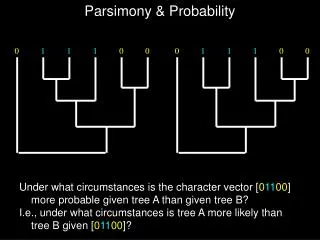
Parsimony & Probability Under what circumstances is the character vector [01100] more probable given tree A than given tree B? I.e., under what circumstances is tree A more likely than tree B given [01100]?
Parsimony & Probability • P[change] is the same on each branch; • Branch length unimportant: • No rate shifts on tree; • Other characters do not affect probability of change; • P[gain] = P[loss]. • Only a single ancestral reconstruction is considered per node.
Parsimony & Probability Tree A requires only one change.
Parsimony & Probability The probability of the character vector is: P[change]changes x (1-P[change])static branches Log-likelihood of tree is: changes x ln(P[change] + statics x ln(1-P[change])
Parsimony & Probability If P[change] = 0.1, then: P[character | tree] = 0.11 x 0.99 = 3.87 x 10⁻² ln L[tree | character] = ln(0.1) + (9 x ln[0.9]) = -3.25
Parsimony & Probability If P[change] = 0.1, then: P[character | tree] = 0.12 x 0.98 = 4.30 x 10⁻³ ln L[tree | character] = (2 x ln[0.1]) + (8 x ln[0.9]) = -5.45
Parsimony & Probability If P[change] = 0.01, then: P[character | tree] = 0.011 x 0.999 = 9.14 x 10⁻³ ln L[tree | character] = ln(0.01) + (9 x ln[0.99]) = -4.70
Parsimony & Probability If P[change] = 0.01, then: P[character | tree] = 0.012 x 0.998 = 9.23 x 10⁻⁵ ln L[tree | character] = (2 x ln[0.01]) + (8 x ln[0.99]) = -9.29
Parsimony & Probability If P[change] = 0.001, then: P[character | tree] = 0.0011 x 0.9999 = 9.91 x 10⁻⁴ ln L[tree | character] = ln(10-3) + (9 x ln[0.999]) = -6.91
Parsimony & Probability If P[change] = 0.001, then: P[character | tree] = 0.0012 x 0.9998 = 9.92 x 10⁻⁷ ln L[tree | character] = (2 x ln[10-3]) + (8 x ln[0.999]) = -13.82
Infinity and beyond….. P[change] ln L[tree A] ln L[tree B] Difference 10-1 -3.25 -5.45 2.20 10-2 -4.70 -9.29 4.60 10-3 -6.92 -13.82 6.91 10-∞ -∞ -2 x ∞ ∞
Shorter tree is more likely while P[change]<0.5 P[change] ln L[tree A] ln L[tree B] Difference 0.2 -3.62 -5.00 1.62 0.4 -5.51 -5.92 0.41 0.5 -6.93 -6.93 0.00 0.6 -8.76 -8.35 -0.41
Shorter tree is more likely while P[change]<0.5 P[change] ln L[tree A] ln L[tree B] Difference 0.5 -6.93 -6.93 0.00 Shift does not occur at P[change] > 0.15 because only a single way of generating one or two changes is considered.
Relaxing assumptions of parsimony • Low vs. high rates of change. • Homogeneous vs. heterogeneous rates. • Unit vs. variable branch lengths. • Certain vs. uncertainty in ancestral reconstructions. • Independent vs. correlated character change.
Likelihood & phylogeny: some important concepts • Conditional probability: P[X | Z] when X is affected by “intermediate” parameter Y: P[X | Z] = ∑ P[X | Y] x P[Y | Z] • Parameters: some variables can have multiple parameters (e.g., chars. 1-10 have rate i whereas chars. 11-20 have rate k) • Increasing number of differing parameters will increase likelihoods; • Likelihood Ratio tests: used to evaluate whether additional parameters are justified • 2 distribution if hierarchical. • Information theory criteria if non-hierarchicl.
Likelihood & phylogeny: some important concepts • Conditional probability: P[X | Z] when X is affected by “intermediate” parameter Y: P[X | Z] = ∑ P[X | Y] x P[Y | Z] • Parameters: some variables can have multiple parameters (e.g., chars. 1-10 have rate i whereas chars. 11-20 have rate k) • Increasing number of differing parameters will increase likelihoods; • Likelihood Ratio tests: used to evaluate whether additional parameters are justified • 2 distribution if hierarchical. • Information theory criteria if non-hierarchicl.
Likelihood & phylogeny: some important concepts • Conditional probability: P[X | Z] when X is affected by “intermediate” parameter Y: P[X | Z] = ∑ P[X | Y] x P[Y | Z] • Parameters: some variables can have multiple parameters (e.g., chars. 1-10 have rate i whereas chars. 11-20 have rate k) • Increasing number of differing parameters will increase likelihoods; • Likelihood Ratio tests: used to evaluate whether additional parameters are justified • 2 distribution if hierarchical. • Information theory criteria if non-hierarchical.
Advantages of Likelihood • Allows assumptions of parsimony (or other likelihood) analyses to be dissected; • Allows testing of parameters other than phylogeny; • Assumptions plainly stated. • Allows different data types (e.g., morphology / stratigraphy / molecules) to weigh in against hypothesis.
How Likelihood can RejectGeneral Phylogenetic Hypotheses Log Likelihood (Support) µ ln P[data | H] Tree consistent with Hypothesis A. Tree consistent with Hypothesis B.
How Likelihood can RejectGeneral Phylogenetic Hypotheses Log Likelihood (Support) µ ln P[data | H] Tree consistent with Hypothesis A. Tree consistent with Hypothesis B. Note: we might reject B without specifying a particular phylogeny or model of character evolution.
Disadvantages of Likelihood • Much slower than parsimony analyses! • Some hold that parameters assumed to be important in likelihood analyses (e.g., rates, branch lengths, etc.), should be discovered by learning phylogeny, not part of the test for phylogeny.
Effect of Branch Lengths: Felsenstein 1973 • Given a rate and a branch duration of time b, the expected number of changes is b. • Probability of ∆ changes modeled as a Poisson process (i.e., change can occur at any time). (b)∆ x e-(b) • P[∆ | b] = ————— ∆!
Effect of Branch Lengths: Example L[,=0.95| char] = P[0->2|b=0.96] x P[0->0|b=0.96] x P[0->0|b=0.14] x P[0->2|b=1.10] x P[0->0|b=1.10]
Effect of Branch Lengths: Example L[,=0.95| char] = P[0->2|b=0.96] = ([0.95 x 0.96]2 x e-(0.95 x 0.96))/2! x P[0->0|b=0.96] = e-(0.95 x 0.96) x P[0->0|b=0.14] = e-(0.95 x 0.14) x P[0->2|b=1.10] = ([0.95 x 1.10]2 x e-(0.95 x 1.10))/2! x P[0->0|b=1.10] = e-(0.95 x 1.10) = 3.97x10⁻³
Effect of Branch Lengths: Example ln L[,=0.95| char] = ln P[0->2|b=0.96] + ln P[0->0|b=0.96] + ln P[0->0|b=0.14] + ln P[0->2|b=1.10] + ln P[0->0|b=1.10] = -5.53
Effect of Branch Lengths: Example ln L[,=0.95| char] = ln P[0->2|b=0.96] = (2 x ln[0.95 x 0.96])- (0.95 x 0.96) - ln(2) + ln P[0->0|b=0.96] = -(0.95 x 0.96) + ln P[0->0|b=0.14] = -(0.95 x 0.14) + ln P[0->2|b=1.10] = (2 x ln[0.95 x 1.10]- (0.95 x 1.10) - ln(2) + ln P[0->0|b=1.10] = -(0.95 x 1.10) = -5.53
Effect of Branch Lengths: Example L[,=0.95| char] = P[0->2|b=0.96] = ([0.95 x 0.96]2 x e-(0.95 x 0.96))/2! x P[0->0|b=0.96] = e-(0.95 x 0.96) x P[0->0|b=0.14] = e-(0.95 x 0.14) x P[0->2|b=1.10] = ([0.95 x 1.10]2 x e-(0.95 x 1.10))/2! x P[0->0|b=1.10] = e-(0.95 x 1.10) = e-(0.95 x 4.26) x [0.95 x 0.96]2 x [0.95 x 1.10]2/(2!x2!)
Tree Likelihood Rephrased • e-(0.95 x 4.26) x [0.95 x 0.96]2 x [0.95 x 1.10]2 /(2!x2!) • e-(rate x ∑ branches durations) x [rate x branch durations]changesi÷ changes1! for all branches showing change in character. • Log-likelihood there is just: Rate x ∑static branch durations + ∑ changes x ln (rate x branch duration) - ln (changes!) for all branches showing change in the character. • Can it be this easy???
Tree Likelihood Rephrased • e-(0.95 x 4.26) x [0.95 x 0.96]2 x [0.95 x 1.10]2 /(2!x2!) • e-(rate x ∑ branches durations) x [rate x branch durationi]changesi÷ changesi! for all branches showing change in character. • Log-likelihood there is just: Rate x ∑static branch durations + ∑ changes x ln (rate x branch duration) - ln (changes!) for all branches showing change in the character. • Can it be this easy???
Tree Likelihood Rephrased • e-(0.95 x 4.26) x [0.95 x 0.96]2 x [0.95 x 1.10]2 /(2!x2!) • e-(rate x ∑ branches durations) x [rate x branch durationsi]changesi÷ changesi! for all branches showing change in character. • Log-likelihood there is just: Rate x ∑static branch durations + ∑ changes x ln (rate x branch duration) - ln (changes!) for all branches showing change in the character. • Can it be this easy???
Tree Likelihood Rephrased • e-(0.95 x 4.26) x [0.95 x 0.96]2 x [0.95 x 1.10]2 /(2!x2!) • e-(rate x ∑ branches durations) x [rate x branch durationsi]changesi÷ changesi! for all branches showing change in character. • Log-likelihood there is just: Rate x ∑static branch durations + ∑ changes x ln (rate x branch duration) - ln (changes!) for all branches showing change in the character. • Can it be this easy???
What is the likelihood of the 2nd nodes states? L[node 2 = 0| taxa 1, 2] = P[0->2|b=0.96] x P[0->0|b=0.96] L[node 2 = 1| taxa 1, 2] = P[1->2|b=0.96] x P[0->0|b=0.96] L[node 2 = 2| taxa 1, 2] =L[node 2 = 0| taxa 1, 2]
What is the likelihood of the 2nd nodes states? L[node 2 = 0| taxa 1, 2] = 0.067 = P[0->2|b=0.96] = ([0.95 x 0.96]2 x e-(0.95 x 0.96))/2! x P[0->0|b=0.96] = e-(0.95 x 0.96) L[node 2 = 1| taxa 1, 2] = 0.134 = P[1->2|b=0.96] = ([0.95 x 0.96]1 x e-(0.95 x 0.96))/1! x P[0->0|b=0.96] = ([0.95 x 0.96]1 x e-(0.95 x 0.96))/1! L[node 2 = 2| taxa 1, 2] = 0.067
What is the likelihood of the basal nodes states? L[node1 = X| 2, 0, 2, 0] = P[0| node1 = X] x P[2| node1 = X] x (P[0| node1 = X] x P[0 | node2=0] x P[0 | node2=0] + P[1| node1 = X] x P[0 | node2=1] x P[0 | node2=1] + P[2| node1 = X] x P[0 | node2=2] x P[0 | node2=2])
What is the likelihood of the basal nodes states? L[node1 = X| 2, 0, 2, 0] = P[0| node1 = X] x P[2| node1 = X] x (P[0| node1 = X] x P[0 | node2=0] x P[0 | node2=0] + P[1| node1 = X] x P[0 | node2=1] x P[0 | node2=1] + P[2| node1 = X] x P[0 | node2=2] x P[0 | node2=2]) Note: final terms are the likelihoods of node 2 states times the conditional probabilities of those states given node 1.
Ancestral conditions as conditional probability L[,=0.95| 2, 0, 2, 0] = 0 x L[node1 = 0| 2, 0, 2, 0] + 1 x L[node1 = 1| 2, 0, 2, 0] + 2 x L[node1 = 2| 2, 0, 2, 0] Where i is the probability of beginning with state i. Tree likelihood obviously modified.
Phylogeny Likelihood characters states branches • L[, | C] = ∑ P[∆ijk | bj, ] i=1 k=0 j=1 • : rate; • b: branch j on tree • C: character matrix • ∆ijk: number of changes in character i on branch j given ancestral state k. • Different phylogenies matching the same cladogram will have different likelihoods!
Changing Branch Durations Changes Likelihood Likelihood of upper node as well as P[0], P[1] or P[2] red, yellow and orange branches now altered. Sum of potentially static lineages AND lineages over which change accrued also differ on the two trees. Upshot: cladogram does not have likelihood unless you sum over all possible phylogenies!
With fossils, adding unsampled ancestors increases likelihood. Hypothetical ancestors decrease necessary transitions and increase possible pathways.
With fossils, adding unsampled ancestors increases likelihood. If P[∆] = 0.05, then L[1] = 0.052 = 2.5x10⁻³
With fossils, adding unsampled ancestors increases likelihood. L[2] = 0 x (L[2A] + L[2B]) + 1 x (L[2A] + L[2B]) where i is the probability of state i at the base.
With fossils, adding unsampled ancestors increases likelihood. L[2A] = 0.95 x 0.05 x 0.95 x 0.95 = 4.29 x 10⁻²
With fossils, adding unsampled ancestors increases likelihood. L[2B] = 0.05 x 0.95 x 0.95 x 0.05 = 2.26 x 10⁻³
With fossils, adding unsampled ancestors increases likelihood. L[2C] = 0.05 x 0.05 x 0.05 x 0.95 = 1.19 x 10⁻⁴
With fossils, adding unsampled ancestors increases likelihood. L[2D] = 0.05 x 0.95 x 0.95 x 0.05 = 2.26 x 10⁻³
With fossils, adding unsampled ancestors increases likelihood. If P[∆] = 0.05, then L[1] = 2.5x10⁻³ L[2] ≅ 2.4x10⁻²
Changing Rate Changes Likelihood First tree’s likelihood maximized at ≅ 0.95; Second tree’s likelihood maximized at ≅ 1.20; Same number of changes favored, but less time: (t= 4.26 vs. t = 3.30) Upshot: cladogram does not have likelihood unless you sum over all possible rates!
Continuous vs. Pulsed Change • Equations presented above assume continuous change. • What if change is pulsed? (speciational, punctuated, etc.); • If so, then change should have a binomial distribution at each pulse; • However, pulses themselves might have a Poisson distribution • e.g., based on speciation rate. • This gives a Poisson distribution of binomial events! anc • P[∆ | t] = ∑P[∆ | i species, ] x P[i species | µ, t], i=1 • µ = speciation rate, • t = time; • anc = unsampled ancestral species.
“Weights” and likelihood Doubling a character’s weight invokes two step matrices: From\To: 0 1 From\To: 0 1 0 0 1 0 0 2 1 1 0 1 2 0 This assumes that P[change char. B] = P[change char. A]2, not P[change char. B] = 2 x P[change char. A]. From\To: 0 1 From\To: 0 1 0 1-pa pa 0 1-(pa)2 (pa)2 1 pa 1-pa 1 (pa)2 1-(pa)2 Thus, weights reflect exponents of “base” rate.
“Ordered states” and likelihood Doubling a character’s weight invokes two step matrices: From\To: 0 1 2 0 0 1 2 1 1 0 1 2 2 1 0 Instead of implying that 1 must evolve between 0 and 2, it now implies that P[0<->1] = P[0<->2]2. From\To: 0 1 2 0 1-(p+p2) p p2 1 p 1-2p p 2 p2 p 1-(p+p2) Note: Each row must sum to 1.0.