A Multiscale CCTA plus Spectral Graph Partitioning for Image Segmentation
320 likes | 510 Vues
A Multiscale CCTA plus Spectral Graph Partitioning for Image Segmentation. 报告人:周静波. 2011 年 8 月 25 日. Outline. Related works C onnected C oherence T ree A lgorithm Motivation The proposed algorithm Experiment. Image Segmentation.

A Multiscale CCTA plus Spectral Graph Partitioning for Image Segmentation
E N D
Presentation Transcript
A Multiscale CCTA plus Spectral Graph Partitioning for Image Segmentation 报告人:周静波 2011年8月25日
Outline Related works Connected Coherence Tree Algorithm Motivation The proposed algorithm Experiment
Image Segmentation Image segmentation is the most challenging and critical problem in image processing and analysis. finding the faint object boundaries separating the highly cluttered background
Related Works Clustering based methods unable to handle unbalanced elongated clusters Histogram based methods cannot separate those areas which have the same gray level but do not belong to the same part Region growing methods depend on the seed seriously Graph based methods depends mainly on the graph affinities which affected by the graph connection radius seriously
Related Works Multiscale image segmentation frameworks give efficient approximation to incorporate long-range connections with low complexity fail to detect fine-level details along object boundaries Region-based method Why not integrates multiscale image segmentation framework and region-based method into a new framework?
Connected Coherence Tree Algorithm An image is a pair --- a finite set of pixels ---a mapping---assigns to each pixel a pixel value in some arbitrary value space For a fixed pixel , we define its neighborhood as
Connected Coherence Tree Algorithm Given an arbitrary threshold , pixels in can divided into two different sets Then we can define one neighborhood coherence factor (NCF) as follows:
Connected Coherence Tree Algorithm Note that, is similar to most of its neighboring pixels when
Connected Coherence Tree Algorithm Choose the pixels, whose NCF is larger than 0.5, as seed to grow the region. Choose any seed to start . t p r s q
Parameters Spatial scale k and the intensity difference scale We calculate the average of , as a candidate for
Connected Coherence Tree Algorithm We give an example k=20 k=15 k=10 k=6
Connected Coherence Tree Algorithm Some problem with CCTA the quality of segmentation depend on the parameters the number of clusters cannot set by prior information
Motivation k is related to the size of the objects of interest in the image Run CCTA with different scales, then combine the results together. when k is large when k is small big computational complexity small computational complexity How to produce the segment result with coarse- and fine-level details ? under-segmentation over-segmentation retain the coarse-level details retain the fine-level details
The proposed algorithm Run CCTA with multiple scales, obtain the segment regions . Design a graph The weight matrix is defined as follows
The proposed algorithm W* can berewritten as A is a connectivity matrix whose rows corresponding to the pixels and columns corresponding to the regions The advantage of W* If a segment with new scale is added, a new set of regions will be added to the graph easily. W is a sparse matrix and easy to partition.
The proposed algorithm Use spectral graph partitioning algorithm after the weight matrix constructed. A. Ng, M. Jordan, and Y. Weiss. On spectral clustering: Analysis and an algorithm. Advances in Neural Information Processing Systems 14. MIT Press, 2002, pp.849-856 Output the label of pixels as final result.
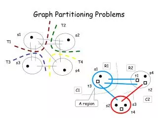
An example Region 1 Region 2 Scale 1 region 1 region 2 Scale 2 Region 3 Region 4 region 3 region 4 Fig.3. An example of MCCTSGP formulation. (a) Regions generated by two scales of CCTA. (b) We can use red dashed line to cut one of edges to form two parts, region 1 and region 3, region 2 and region 4, according to spectral graph partitioning objective function, respectively.
How to choose parameters There are two kinds of parameters the group scales the number of segments For group scales How to choose the spatial scale k? How many scales used in MCCTSGP?
How to choose parameters As mentioned in CCTA, an optimal k would be in the range [5, 15].To obtain regions with large difference, we get k from the range [5, 30] that covers the range of optimum Choose more scales obtain more regions that make sure the accuracy of final segmentation requires much more computational cost
Experiment Berkeley image database contains 300 images and their corresponding ground truth data Parameters In visual performance The number of class set it according to the annotation or the contends of the image.
Experiment Compare to Conventional Methods: CCTA (Ding J, Ma R, Chen S. A Scale-based coherence connected tree algorithm for image segmentation. IEEE Trans. on Image Proc.,2008) CTM---a region-based segmentation algorithm Allen Yang, John Wright, Yi Ma, and Shankar Sastry. Unsupervised Segmentation of Natural Images via Lossy Data Compression, Computer Vision and Image Understanding (CVIU), Vol.110, Issue2 (2008) NCut---a spectral graph segmentation algorithm (J. Shi and J. Malik. Normalized cuts and image segmentation. IEEE Trans. on PAMI, 2000.) MNCut---a multiscale image segmentation algorithm (T.Cour, F.Benezit, and J.Shi. Spectral segmentation with multiscale graph decomposition. In Proc. CVPR 2005)
Visual performance NCut CCTA CTM New MNCut
Visual performance CCTA CTM NCut MNCut New Fig.4. Examples in category animals.
Visual performance CCTA CTM NCut MNCut New Fig.7. Examples in category landscape and building.
Visual performance CCTA CTM NCut MNCut New Fig. 6. Examples in category sporting scene
Quantitative performance The Probabilistic Rand Index (PRI) counts the fraction of pairs of pixels whose labels are consistent between the computed segmentation and the ground truth, averaging across multiple ground truth segmentations to account for scale variation in human perception The Variation of Information (VoI) defines the distance between two segmentations as the average conditional entropy of one segmentation given the other, and thus roughly measures the amount of randomness in one segmentation which cannot be explained by the other. The Global Consistency Error (GCE) measures the extent to which one segmentation can be viewed as a refinement of the other. The Boundary Displacement Error (BDE) measures the average displacement error of boundary pixels between two segmented images.
Quantitative performance Average performance on Berkley segmentation database (bold indicates best of all the algorithms) ▲----k= ★ -----k=
Quantitative performance Fig 1 Our statistics on Probabilistic Rand Index (PRI), over the Berkeley database with K = {5, 10, 15, ..., 40}, compared with NCut and MNCut, k=
Quantitative performance Fig 9 Our statistics on Variation of Information (VoIover the Berkeley database with K = {5, 10, 15, ..., 40}, compared with NCut and MNCut, k=
Quantitative performance Fig 9 Our statistics on Global Consistency Error (GCEover the Berkeley database with K = {5, 10, 15, ..., 40}, compared with NCut and MNCut, k=
Quantitative performance Fig 9 Our statistics on Boundary Displacement Error (BDE) over the Berkeley database with K = {5, 10, 15, ..., 40}, compared with NCut and MNCut,k=
谢谢! 报告人:姓 名 2011年8月25日