The Challenges of Linkage Analysis in Genetics: Bias, Odds, and Multiple Testing
This document explores the complexities of linkage analysis in genetics, focusing on recombination distances between markers and trait loci. Discussing simulation methods and the implications of bias in coin-flipping analogies, the text illustrates how multiple testing can lead to false positives. It highlights the significance of marker density and LOD scores, emphasizing the necessity of simulations tailored to specific research contexts. Additionally, the piece critiques common approaches like candidate gene strategies and their effectiveness in uncovering genetic relationships.

The Challenges of Linkage Analysis in Genetics: Bias, Odds, and Multiple Testing
E N D
Presentation Transcript
A1 A1 D d A2 A2 d D Dad phase unknown odds ratio Odds = 1/2[(1-r)n • rk] + 1/2[(1-r)n • rk] 0.5(total # meioses) What single r value best explains the data? or A1 A2
For this, you need to search r’s. maximum likelihood r = 0.13 Oops: a numerical mistake (thanks to Jonathan for detective work)
In real life this correction does matter… family 1: 10 meioses, 1 (or 9) apparent recombinants family 2: 10 meioses, 4 (or 6) apparent recombinants family 3: 10 meioses, 3 (or 7) apparent recombinants family 4: 10 meioses, 3 (or 7) apparent recombinants total LOD = LOD(family 1) + LOD(family 2) + LOD(family 3) + LOD(family 4) Accounting for both phases Using only one phase best r = 0.2771 best r = 0.2873
Locus heterogeneity age of onset
Coins r = intrinsic probability of coming up heads (bias) Odds = P(your flips | r) P(your flips | r = 0.5) Odds = (1-r)n • rk 0.5(total # flips) Odds ratio of model that coin is biased, relative to null
Coins r = intrinsic probability of coming up heads (bias) 0 heads 1 heads 2 heads 3 heads 4 heads
Significance cutoff (single family)
The analogy again Testing lots of markers for linkage to a trait is analogous to having lots of students, each flipping a coin. The search for the coin’s bias parameter is analogous to the search for recombination distance between markers and disease locus.
The analogy again Testing lots of markers for linkage to a trait is analogous to having lots of students, each flipping a coin. The search for the coin’s bias parameter is analogous to the search for recombination distance between markers and disease locus. Each student is analogous to a marker.
The analogy again Testing lots of markers for linkage to a trait is analogous to having lots of students, each flipping a coin. The search for the coin’s bias parameter is analogous to the search for recombination distance between markers and disease locus. Each student is analogous to a marker. Each coin flip is analogous to a family member in pedigree.
Multiple testing, shown another way 1. Simulate thousands of markers, inherited from parents to progeny. 2. Assign some family members to have a disease, others not. 3. Test for linkage between disease and markers, knowing there is none. E. Lander and L. Kruglyak, Nature Genetics 11:241, 1995
Simulation Every marker is analogous to a student flipping
A real world scenario You have invested a bolus of research money in a linkage mapping study of a genetic disease segregating in families. For each family member, you do genotyping at a bunch of markers. When you finally run the linkage calculation, the strongest marker gives a LOD of 2. You desperately want to believe this is significant. You simulate a fake trait with no genetic control 1000 times. You find that in 433 of these simulations, the fake trait had a LOD > 2. This means that in your real data, the probability of your precious linkage peak being a false positive is 433/1000 = 0.433. If you spent more money and time to follow this up, it could be a complete waste. Essential to know.
Simulation/theory Simulate 1000 times, ask how frequently you get a peak over a certain threshold.
Simulation/theory With modest marker spacing in a human study, LOD of 3 is 9% likely to be a false positive.
Simulation/theory But this would change in a different organism, with different number of markers, etc.
Simulation/theory But this would change in a different organism, with different number of markers, etc. So in practice, everyone does their own simulation specific to their own study.
More markers = more tests = more chance for spurious high linkage score.
More markers = more tests = more chance for spurious high linkage score. Not true when you add individuals (patients)! Always improves results.
Multiple testing in genetics Multiple markers not necessary
Marker density matters ? But if the only marker you test is >50 cM away, will get no linkage.
Marker density matters ? But if the only marker you test is >50 cM away, will get no linkage. So a mapping experiment is a delicate balance between too much testing and not enough…
Candidate gene approach: apple pigment http://waynesword.palomar.edu/images/apple3b.jpg
Candidate gene approach Hypothesize that causal variant will be in known pigment gene or regulator. NOT randomly chosen markers genome-wide.
Candidate gene approach Red progeny have RFLP pattern like red parent
Candidate gene approach Unpigmented progeny have RFLP pattern like unpigmented parent
But if you can beat multiple testing, why not do the whole genome…
Testing for linkage doesn’t always mean counting recombinants.
Back to week 4 Fig. 3.12
Qualitative but polygenic Two loci. Need one dominant allele at each locus to get phenotype. Fig. 3.12
A simulated cross: test one locus AAbb aaBB inter-mate AaBb Two loci. Need one dominant allele at each locus to get phenotype. Flower color Genotype at marker close to A locus
A simulated cross: test one locus AAbb aaBB inter-mate AaBb Two loci. Need one dominant allele at each locus to get phenotype. AaBb aaBB AABb aaBb AaBB Aabb Flower color Genotype at marker close to A locus
A simulated cross: test one locus AAbb aaBB inter-mate AaBb Two loci. Need one dominant allele at each locus to get phenotype. AaBb aaBB AABb aaBb AaBB Aabb Flower color Genotype at marker close to A locus
A simulated cross: test one locus AAbb aaBB inter-mate AaBb Two loci. Need one dominant allele at each locus to get phenotype. AaBb aaBB AABb aaBb AaBB Aabb Purple flowers result from AA or Aa. Flower color Genotype at marker close to A locus
No need to count recombinants AAbb aaBB inter-mate AaBb Two loci. Need one dominant allele at each locus to get phenotype. AaBb aaBB AABb aaBb AaBB Aabb Flower color Genotype at marker close to A locus
No need to count recombinants AAbb aaBB inter-mate AaBb Two loci. Need one dominant allele at each locus to get phenotype. AaBb aaBB AABb aaBb AaBB Aabb 2 = (O - E)2 Flower color E Genotype at marker close to A locus
No need to count recombinants AAbb aaBB inter-mate AaBb Two loci. Need one dominant allele at each locus to get phenotype. AaBb aaBB AABb aaBb AaBB Aabb NOT complete co-inheritance. Flower color Genotype at marker close to A locus
“A weak locus” Because A locus by itself is not the whole story, studying it in isolation gives only weak statistical significance. Two loci. Need one dominant allele at each locus to get phenotype. 2 = (O - E)2 E
Many traits—cancers, cleft palate, high blood pressure—fit this description.
Multiple loci underlie many yes-or-no traits % individuals “Threshold model”
Multiple loci underlie many yes-or-no traits % individuals “Threshold model” Number of disease-associated alleles a person has, combined across all loci
Affected sib pair method 2,2 2,3 2,2 2,2
Affected sib pair method 2,2 2,3 What is probability of this by chance? 2,2 2,2 Both kids affected, both got allele 2 at marker from mom. 1/4 1/2 1/8 1/3
Affected sib pair method 2,2 2,3 What is probability of both kids getting 2 from mom or both kids getting 3 from mom? 2,2 2,2 Both kids affected, both got allele 2 at marker from mom. 1/4 1/2 1/8 1/3
Affected sib pair method 2,2 2,3 What is probability of both kids getting 2 from mom or both kids getting 3 from mom? 2,2 2,2 Both kids affected, both got allele 2 at marker from mom. 1/4 1/2 1/8 1/3 (1/2)*(1/2) + (1/2)*(1/2) Prob of both getting 2 Prob of both getting 3