Review of Sequential Representations

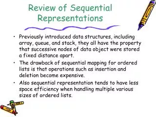
1. Review of Sequential Representations • Previously introduced data structures, including array, queue, and stack, they all have the property that successive nodes of data object were stored a fixed distance apart. • The drawback of sequential mapping for ordered lists is that operations such as insertion and deletion become expensive. • Also sequential representation tends to have less space efficiency when handling multiple various sizes of ordered lists.

2. Linked List • A better solutions to resolve the aforementioned issues of sequential representations is linked lists. • Elements in a linked list are not stored in sequential in memory. Instead, they are stored all over the memory. They form a list by recording the address of next element for each element in the list. Therefore, the list is linked together. • A linked list has a head pointer that points to the first element of the list. • By following the links, you can traverse the linked list and visit each element in the list one by one.

3. Linked List Insertion • To insert an element into the three letter linked list: • Get a node that is currently unused; let its address be x. • Set the data field of this node to GAT. • Set the link field of x to point to the node after FAT, which contains HAT. • Set the link field of the node cotaining FAT to x.

4. Linked List Insertion And Deletion first CAT BAT EAT FAT HAT GAT first CAT BAT EAT FAT GAT HAT

5. Pointer Manipulation in C++ x a y b • Addition of integers to pointer variable is permitted in C++ but sometimes it has no logical meaning. • Two pointer variables of the same type can be compared. • x == y, x != y, x == 0 x a b x y b b y x = y *x = * y

6. Circular Lists • By having the link of the last node points to the first node, we have a circular list. • Need to make sure when current is pointing to the last node by checking for current->link == first. • Insertion and deletion must make sure that the circular structure is not broken, especially the link between last node and first node.

7. Diagram of A Circular List first last

8. Linked Stacks and Queues top front rear 0 Linked Queue 0 Linked Stack

9. Revisit Polynomials 1 a.first 14 0 8 3 0 2 6 10 b.first 14 0 8 10 -3

10. Operating On Polynomials • With linked lists, it is much easier to perform operations on polynomials such as adding and deleting. • E.g., adding two polynomials a and b a.first 1 0 14 0 8 3 2 p 6 10 14 0 8 b.first 10 -3 q (i) p->exp == q->exp c.first 0 14 11

11. Operating On Polynomials a.first 1 0 14 0 8 3 2 p 6 10 14 0 8 b.first 10 -3 q c.first 0 14 0 11 10 -3 (ii) p->exp < q->exp

12. Operating On Polynomials 0 14 11 a.first 1 0 14 0 8 3 2 p 6 10 14 0 8 b.first 10 -3 q c.first 10 -3 0 8 2 (iii) p->exp > q->exp

13. Memory Leak • When polynomials are created for computation and then later on out of the program scope, all the memory occupied by these polynomials is supposed to return to system. But that is not the case. Since ListNode<Term> objects are not physically contained in List<Term> objects, the memory they occupy is lost to the program and is not returned to the system. This is called memory leak. • Memory leak will eventually occupy all system memory and causes system to crash. • To handle the memory leak problem, a destructor is needed to properly recycle the memory and return it back to the system.

14. Free Pool • When items are created and deleted constantly, it is more efficient to have a circular list to contain all available items. • When an item is needed, the free pool is checked to see if there is any item available. If yes, then an item is retrieved and assigned for use. • If the list is empty, then either we stop allocating new items or use new to create more items for use.

15. Using Circular Lists For Polynomials • By using circular lists for polynomials and free pool mechanism, the deleting of a polynomial can be done in a fixed amount of time independent of the number of terms in the polynomial.

16. Deleting A Polynomial with a Circular List Structure av 3 a.first 1 0 14 8 3 2 1 second 2 av

17. Equivalence Class • For any polygon x, x ≡ x. Thus, ≡ is reflexive. • For any two polygons x and y, if x ≡ y, then y ≡ x. Thus, the relation ≡ is symetric. • For any three polygons x, y, and z, if x ≡ y and y ≡ z, then x ≡ z. The relation ≡ is transitive.

18. Equivalence Definition: A relation ≡ over a set S, is said to be an equivalence relation over S iff it is symmetric, reflexive, and transitive over S. Example: Supposed 12 polygons 0 ≡ 4, 3 ≡ 1, 6 ≡ 10, 8 ≡ 9, 7 ≡ 4, 6 ≡ 8, 3 ≡ 5, 2 ≡ 11, and 11 ≡ 0. Then they are partitioned into three equivalence classes: {0, 2, 4, 7, 11}; {1 , 3, 5}; {6, 8, 9 , 10}

19. Equivalence (Cont.) • Two phases to determine equivalence • In the first phase the equivalence pairs (i, j) are read in and stored. • In phase two, we begin at 0 and find all pairs of the form (0, j). Continue until the entire equivalence class containing 0 has been found, marked, and printed. • Next find another object not yet output, and repeat the above process.

20. Equivalence Definition: A relation ≡ over a set S, is said to be an equivalence relation over S iff it is symmetric, reflexive, and transitive over S. Example: Supposed 12 polygons 0 ≡ 4, 3 ≡ 1, 6 ≡ 10, 8 ≡ 9, 7 ≡ 4, 6 ≡ 8, 3 ≡ 5, 2 ≡ 11, and 11 ≡ 0. Then they are partitioned into three equivalence classes: {0, 2, 4, 7, 11}; {1 , 3, 5}; {6, 8, 9 , 10}

21. Equivalence (Cont.) • Two phases to determine equivalence • In the first phase the equivalence pairs (i, j) are read in and stored. • In phase two, we begin at 0 and find all pairs of the form (0, j). Continue until the entire equivalence class containing 0 has been found, marked, and printed. • Next find another object not yet output, and repeat the above process.

22. Equivalence Classes (Cont.) • If a Boolean array pairs[n][n] is used to hold the input pairs, then it might waste a lot of space and its initialization requires complexity Θ(n2) . • The use of linked list is more efficient on the memory usage and has less complexity, Θ(m+n) .

23. Linked List Representation [0] [1] [2] [3] [4] [5] [6] [7] [8] [9] [10] [11] data 11 3 11 5 7 3 8 4 6 8 6 0 link 0 0 0 0 0 0 data 4 1 0 10 9 2 link 0 0 0 0 0 0

24. Linked List for Sparse Matrix • Sequential representation of sparse matrix suffered from the same inadequacies as the similar representation of Polynomial. • Circular linked list representation of a sparse matrix has two types of nodes: • head node: tag, down, right, and next • entry node: tag, down, row, col, right, value • Head node i is the head node for both row i and column i. • Each head node is belonged to three lists: a row list, a column list, and a head node list. • For an nxm sparse matrix with r nonzero terms, the number of nodes needed is max{n, m} + r + 1.

25. Node Structure for Sparse Matrices down tag right down tag row col right f i j next value Head node Typical node Setup for aij A 4x4 sparse matrix

26. Linked Representation of A Sparse Matrix 4 0 1 3 4 2 0 3 H1 H3 H2 H0 Matrix head H0 11 H1 12 2 1 H2 -4 H3 -15

27. Reading In A Sparse Matrix • Assume the first line consists of the number of rows, the number of columns, and the number of nonzero terms. Then followed by num-terms lines of input, each of which is of the form: row, column, and value. • Initially, the next field of head node i is to keep track of the last node in column i. Then the column field of head nodes are linked together after all nodes has been read in.

28. Complexity Analysis • Input complexity: O(max{n, m} + r) = O(n + m + r) • Complexity of ~Maxtrix(): Since each node is in only one row list, it is sufficient to return all the row lists of a matrix. Each row is circularly linked, so they can be erased in a constant amount of time. The complexity is O(m+n).

29. Doubly Linked Lists • The problem of a singly linked list is that supposed we want to find the node precedes a node ptr, we have to start from the beginning of the list and search until find the node whose link field contains ptr. • To efficiently delete a node, we need to know its preceding node. Therefore, doubly linked list is useful. • A node in a doubly linked list has at least three fields: left link field (llink), a data field (item), and a right link field (rlink).

30. Doubly Linked List • A head node is also used in a doubly linked list to allow us to implement our operations more easily. rlink item llink Head Node rlink item llink Empty List

31. Deletion From A Doubly Linked Circular List rlink item llink Head Node

32. Insertion Into An Empty Doubly Linked Circular List node node newnode