Data, Calibration and Analysis with SOT/HINODE
190 likes | 215 Vues
This guide covers calibration & analysis of SOT/HINODE solar data including SOT FITS format, calibration routines, data catalog checking, & file manipulation using IDL.

Data, Calibration and Analysis with SOT/HINODE
E N D
Presentation Transcript
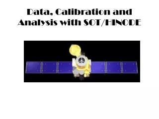
HINODE • Solar Optical Telescope (SOT) • EUV Imaging Spectrometer (EIS) • X-ray Telescope (XRT)
Solar Optical Telescope Optical Telescope assembly specifications
Level-0 Data of Hinode • The Level-0 data are not calibrated. • The fits files are in Level-0 data. • Level -1, 2 obtained after calibrating the data with SSW software, which includes dark subtraction and flat fielding etc. • SOT FITS Data Format http://solar-b.nao.ac.jp/hrc_e/lv0_desc.shtml
Filenames of SOT Level-0 fits files 1. FGyyyymodd_hhmmss.s.fits FGFiltergram. Ex: G-Band, Ca II K, Blue continuum, Na D1 etc. 2. FGIVyyyymodd_hhmmss.s.fits FGIV Shuttered Stokes I and V images. 3.FGSIVyyyymodd_hhmmss.s.fits FGSIVshutterless Stokes-I and V images. 4. FGSIQUVyyyymodd_hhmmss.s.fits FGSIQUV shutter less Stokes I, Q, U & V images. 5. SP4Dyyyymodd_hhmmss.s.fits The Stokes spectrum data (SOT-SP), 4D Stokes I, Q, U & V. The unit of the file is one slit position, not one raster. yyyy:Year, mo:Month, dd:Day, hh:Hour, mm:Minutes ss/ss.s:Second
Examples of SOT/FG filenames • Each data sets are arranged under the subdirectory/hinode/sot/level0/year/month/date/FG/hour/filenames Ex:/disk/jf1/HINODE/sot/level0/2006/12/28/FG/H0000 /disk/jf1/HINODE/sot/level0/2006/12/28/FGIQUV/H1700 /disk/jf1/HINODE/sot/level0/2006/12/28/SP4D/H0000 • Filenames of Level-0 data. Ex: 1. FG20061228_00253332.2.fits 2. FGIQUV20061228_170032.1.fits 3. FGIV20061228_103518.2.fits 4. FGSIQUV20061228_170212.5.fits 5. SP4D20061228_00645.4.fits
Routines to calibrate the FG/SOT data • To check the SOT data catalog. idl> sot_cat,'2006-10-28','2006-10-29',sotcatTo check the available data between 2006-10-28 to 2006-10-29, the structure sotcat contains the information. Then one can use the following routine to see the files. idl>files = sot_cat2files(sotcat)All the names of the files and their paths are stored in files. Idl>read_sot,files,index,dataTo read those files use the routine read_sot and the calling sequence is as above. Idl>sot_cat,'28-Dec-06 15:00','28-Dec-06 18:00',index,files,/level0One can use the above arguments to check the data between 15:00 – 18:00 UT of 28th December 2006. The file names and their paths are stored in files. • To read and calibrate the broad-band image data. idl> file = findfile(‘*.fits’) idl> mreadfits, file,index idl> ss = where(index.WAVE eq ‘Ca II H line’) Or Index.Wave eq ‘G band 4305’ or ‘CN bandhead 3883’ or ‘blue cont 4504’ or ‘red cont 6684’ or ‘green cont 5550’ Idl>fg_prep,file(ss),index_out,image_out,/despike,/display,/float,/verbose,/tf_deripple,/outflatfits,outdir=‘/disk/data/ravindra/hinode/’ Process an SOT BFI or NFI filtergram, magnetogram, dopplergram, or Stokes set despike - cosmic ray removal, /no_flat - skip flat fielding (This option is necessary for NFI.), /float - return images with floating (default: integer), /quiet - set for fewer messgaes, /verb - set for lots of messages Idl> write_sot,index_out,data_out
Rigid Alignment of the FG images idl>fileb = findfile('reg20070406_*.fits') idl> mreadfits,fileb,indexb,datab Idl> fg_rigidalign, indexb, datab, index_outb, data_outb, dx = 512, dy =512, x0 = 10, y0 = 10, nt = 40 dx=the x-dimension of the box in which image-to-image correlations are calculated. Default = 256. dy=the y-dimension of the box in which image-to-image correlations are calculated. ; Default = 256. X0: the x-coordinate of the lower-left corner of the correlation box. ; Default = image center. ; Y0: the y-coordinate of the lower-left corner of the correlation box. ; Default = image center. ; Nt: the number of images correlated at one time, i.e. the number of images ; assembled into a subgroup and aligned with respect to the first image in the group. ; Default = 4. Set this parameter to be less than the number of images over which the ; correlated structures in the images change significantly. To make a movie Idl>xstepper,data [,info_array , xsize=xsize, ysize=ysize, /interp ,start=start, /noscale] make Hinode SOT/XRT movies for given time range ; hinode_make_wwwmovies.pro
Programs to calibrate the SP/SOT level0 data idl> file=sot_filelist(obs,start_time,end_time,topdir=topdir0,/scanset, sltidx=sltidx,macroid=macroid,sp_end=sp_end) ;extract file list from level-0/1 data tree idl> dir=sot_filelist(‘SP4D','20061124_010000','20061124_032000') ; =>extract SP4D data directory between start_time and end_time idl>file=findfile(‘./SP4D20070406*.fits’) idl>sp_prep,file,index,ldata,/display,outdir=‘/hinode/apr0607/’ File = array of file pathnames for one operation. Index, ldata= return index(header) and data(*,*,4). Input file size: Ex: Filename: SP4D20070302_161839.2.fits DATA INT = Array[112, 512, 2, 4] Calibrated data: ex: SP4D20070302_161839.2C.fits DATA INT = Array[112, 512, 4]
Inversion of Stokes signal to vector magnetic field • Community inversion codes:http://www.hao.ucar.edu/public/research/cic/index.html(1)LILIA v3.1(2) MELANIE v2.01 (3) DIANNE v0.9 (BETA!) Wavelength = ((findgen (112) - index(0).crpix1) * abs (index(0).cdelt1) + index(0).crval1) Co-ordinate of the reference pixel Wavelength of the reference pixel Spectral res.
THREE DATA ARCHIVES http://sot.lmsal.com/sot-data http://darts.isas.jaxa.jp/hinode http://kurasuta.cfa.harvard.edu/VSO Thank You
SP-Mapping mode Dynamic Mode Deep Magnetogram
Spectro-Polarimeter Mapping mode Normal map Fast Map
Tunable filter bubble Tunable elements which carries the bubbles are identified. TF6 big bubble TF5 ~1A TF Bubble in the FOV TF7 Small bubbles
