Correlation and Regression
Correlation and Regression. Correlation. A quantitative relationship between two interval or ratio level variables. Explanatory (Independent) Variable. Response (Dependent) Variable. y. x. Hours of Training. Number of Accidents. Shoe Size. Height . Cigarettes smoked per day.
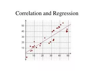

Correlation and Regression
E N D
Presentation Transcript
Correlation A quantitative relationship between two interval or ratio level variables Explanatory (Independent) Variable Response (Dependent) Variable y x Hours of Training Number of Accidents Shoe Size Height Cigarettes smoked per day Lung Capacity Score on SAT Grade Point Average Height IQ What type of relationship exists between the two variables and is the correlation significant?
Correlation • measures and describes the strength and direction of the relationship • Bivariate techniques requires two variable scores from the same individuals (dependent and independent variables) • Multivariate when more than two independent variables (e.g effect of advertising and prices on sales) • Variables must be ratio or interval scale
Scatter Plots and Types of Correlation 60 50 40 30 20 10 0 0 2 4 6 8 10 12 14 16 18 20 x = hours of training (horizontal axis) y = number of accidents (vertical axis) Accidents Hours of Training Negative Correlation–as x increases, y decreases
Scatter Plots and Types of Correlation x = SAT score y = GPA 4.00 3.75 3.50 3.25 GPA 3.00 2.75 2.50 2.25 2.00 1.75 1.50 300 350 400 450 500 550 600 650 700 750 800 Math SAT Positive Correlation–as x increases, y increases
Scatter Plots and Types of Correlation x = height y = IQ 160 150 140 130 IQ 120 110 100 90 80 60 64 68 72 76 80 Height No linear correlation
Scatter Plots and Types of Correlation Strong, negative relationship but non-linear!
1 –1 0 Correlation Coefficient “r” A measure of the strength and direction of a linear relationship between two variables The range of r is from –1 to 1. If r is close to –1 there is a strong negative correlation. If r is close to 1 there is a strong positive correlation. If r is close to 0 there is no linear correlation.
Outliers..... Outliers are dangerous Here we have a spurious correlation of r=0.68 without IBM, r=0.48 without IBM & GE, r=0.21
Application Final Grade Absences x y 8 78 2 92 5 90 12 58 15 43 9 74 6 81 95 90 85 80 75 Final Grade 70 65 60 55 50 45 40 0 2 4 6 8 10 12 14 16 Absences X
Computation of r xy xy y2 x2 624 184 450 696 645 666 486 64 4 25 144 225 81 36 6084 8464 8100 3364 1849 5476 6561 1 8 78 2 2 92 3 5 90 4 12 58 5 15 43 6 9 74 7 6 81 57 516 3751 579 39898
Hypothesis Test for Significance r is the correlation coefficient for the sample. The correlation coefficient for the population is (rho). For a two tail test for significance: (The correlation is not significant) (The correlation is significant) The sampling distribution for r is a t-distribution with n – 2 d.f. Standardized test statistic
Test of Significance The correlation between the number of times absent and a final grade r = –0.975. There were seven pairs of data.Test the significance of this correlation. Use = 0.01. 1. Write the null and alternative hypothesis. (The correlation is not significant) (The correlation is significant) 2. State the level of significance. = 0.01 3. Identify the sampling distribution. A t-distribution with 5 degrees of freedom
df\p 0.40 0.25 0.10 0.05 0.025 0.01 0.005 0.0005 1 0.324920 1.000000 3.077684 6.313752 12.70620 31.82052 63.65674 636.6192 2 0.288675 0.816497 1.885618 2.919986 4.30265 6.96456 9.92484 31.5991 3 0.276671 0.764892 1.637744 2.353363 3.18245 4.54070 5.84091 12.9240 4 0.270722 0.740697 1.533206 2.131847 2.77645 3.74695 4.60409 8.6103 5 0.267181 0.726687 1.475884 2.015048 2.57058 3.36493 4.03214 6.8688 4.032 –4.032 Rejection Regions Critical Values ± t0 t 0 4. Find the critical value. 5. Find the rejection region. 6. Find the test statistic.
t 0 –4.032 +4.032 7. Make your decision. t = –9.811 falls in the rejection region. Reject the null hypothesis. 8. Interpret your decision. There is a significant negative correlation between the number of times absent and final grades.
The Line of Regression Regression indicates the degree to which the variation in one variable X, is related to or can be explained by the variation in another variable YOnce you know there is a significant linear correlation, you can write an equation describing the relationship between the x and y variables. This equation is called the line of regression or least squares line. The equation of a line may be written as y = mx + b where m is the slope of the line and b is the y-intercept. The line of regression is: The slope m is: The y-intercept is:
(xi,yi) = a data point = a point on the line with the same x-value = a residual Best fitting straight line 260 250 240 230 revenue 220 210 200 190 180 1.5 2.0 2.5 3.0 Ad $
xy x2 y2 xy Write the equation of the line of regression with x = number of absences and y = final grade. 1 8 78 2 2 92 3 5 90 4 12 58 5 15 43 6 9 74 7 6 81 624 184 450 696 645 666 486 64 4 25 144 225 81 36 6084 8464 8100 3364 1849 5476 6561 Calculate m and b. 516 3751 579 39898 57 The line of regression is: = –3.924x + 105.667
0 2 4 6 8 10 12 14 16 The Line of Regression m = –3.924 and b = 105.667 The line of regression is: 95 90 85 Grade 80 75 70 65 Final 60 55 50 45 40 Absences Note that the point = (8.143, 73.714) is on the line.
Predicting y Values The regression line can be used to predict values of y for values of x falling within the range of the data. The regression equation for number of times absent and final grade is: = –3.924x + 105.667 Use this equation to predict the expected grade for a student with (a) 3 absences (b) 12 absences = –3.924(3) + 105.667 = 93.895 (a) = –3.924(12) + 105.667 = 58.579 (b)
Strength of the Association The coefficient of determination, r2,measures the strength of the association and is the ratio of explained variation in y to the total variation in y. The correlation coefficient of number of times absent and final grade is r = –0.975. The coefficient of determination is r2 = (–0.975)2 = 0.9506. Interpretation: About 95% of the variation in final grades can be explained by the number of times a student is absent. The other 5% is unexplained and can be due to sampling error or other variables such as intelligence, amount of time studied, etc.