Ch 2: probability sampling, SRS
Ch 2: probability sampling, SRS. Overview of probability sampling Establish basic notation and concepts Population distribution of Y : object of inference Sampling distribution of an estimator under a design: assessing the quality of the estimate used to make inference

Ch 2: probability sampling, SRS
E N D
Presentation Transcript
Ch 2: probability sampling, SRS • Overview of probability sampling • Establish basic notation and concepts • Population distribution of Y : object of inference • Sampling distribution of an estimator under a design: assessing the quality of the estimate used to make inference • Apply these to SRS • Selecting a SRS sample • Estimating population parameters (means, totals, proportions) • Estimating standard errors and confidence intervals • Determining the sample size
Assume ideal setting • Sampled population = target population • Sampling frame is complete and does not contain any OUs beyond the target pop • No unit nonresponse • Measurement process is perfect • All measurements are accurate • No missing data (no item nonresponse) • That is, nonsampling error is absent
Survey error model Total Survey Error Sampling Error Nonsampling Error = + Due to the sampling process (i.e., we observe only part of population) Measurement errorNonresponse errorFrame error Assessed via bias and variance
Probability sample • DEFN: A sample in which each unit in the population has a known, nonzero probability of being included in the sample • Known probability we can quantify the probability of a SU of being included in the sample • Assign during design, use in estimation • Nonzero probability every SU has a positive chance of being included in the sample • Proper survey estimates represent entire target population (under our ideal setting)
Probability sampling relies on random selection methods • Random sampling is NOT a haphazard method of selection • Involves very specific rules that include an element of chance as to which unit is selected • Only the outcome of the probability sampling process (i.e., the resulting sample) is random • More complicated than non-random samples, but provides important advantages • Avoid bias that can be induced by selector • Required to calculate valid statistical estimates (e.g., mean) and measures of the quality of the estimates (e.g., standard error of mean)
Representative sample • Goal is to have a “representative sample” • Probability sampling is used to achieve this by giving each OU in target population an explicit chance to be included in the sample • Sample reflects variability in the population • Applies to the sample, but does not apply to the OU/SU (don’t expect each observation to be a “typical” pop unit • Can create legitimate sample designs that deliberately skew the sample to include adequate numbers of important parts of the variation • Common example: oversampling minorities, women • MUST use estimation procedures that take into account the sample design to make inferences about the target population (e.g., sample weights)
Basic sampling designs • Simple selection methods • Simple random sampling (Ch 2 & 3) • Select the sample using, e.g., a random number table • Systematic sampling (2.6, 5.6) • Random start, take every k-th SU • Probability proportional to size (6.2.3) • “Larger” SU’s have a higher chance of being included in sample • Selection methods with explicit structure • Stratified sampling (Ch 4) • Divide population into groups (strata) • Take sample in every stratum • Cluster sampling (Ch 5 & 6) • OUs aggregated into larger units called clusters • SU is a cluster
Examples • Select a sample of n faculty from the 1500 UNL faculty on campus • Goal: estimate total (or average) number of hours faculty spend per week teaching courses • Simple random sampling (SRS) • Number faculty from 1 to 1500 • Select a set of n random numbers (integers) between 1 and 1500 • Faculty with ids that match the random numbers are included in the sample
Examples - 2 • Systematic sampling (SYS) • Choose a random number between 1 and 1500/n • Select faculty member with that id, and then take every k-th faculty member in the list, with sampling interval k is 1500/n • SRS / SYS • Each faculty member has an equal chance of being included in sample • Each sample of n faculty is equally likely
Examples - 3 • Probability proportional to size (PPS) • With pps design, we assign a selection probability to each faculty member that is proportional to the number of courses taught by a faculty member that semester • “Size” measure = # of courses taught by faculty member • Faculty who teach more courses are more likely to be included in the sample, but those that teach less still have a positive chance of being included • Motivation: faculty that spend more hours on courses are more critical to getting good estimate of total hours spent • Data from faculty with higher inclusion probabilities will be “down weighted” relative to those with lower probabilities during the estimation process • Typically accomplished using weights for each observation in the dataset
Examples - 4 • Stratified random sampling (STS) • Organize list of faculty by college • Stratum = college • Allocate n (divide sample size) among colleges so that we select nh faculty in the h-th college • Sum of nhover strata equals n • Use SRS, e.g., to select sample in each of the college strata • Could use SYS or PPS rather than SRS • Could have different selection methods in each stratum
Examples - 5 • Cluster sampling (CS) • Aggregate faculty into departments • OU = faculty member, SU = dept • Select a sample of departments, e.g., using SRS • Very common to use PPS for selecting clusters • “Size” measure = number of OUs in the the cluster SU • Many variants for cluster sampling • After selecting clusters, may want to select a sample of OUs in the cluster rather than taking data on every OU • E.g., select 15 depts in the first stage of sampling, then select 10 faculty in each dept in a second stage of sampling • This is called 2-stage sampling
Examples - 6 • Complex sample designs (Ch 7) • Combine basic selection methods (SRS, SYS, PPS) with different methods of organizing the population for sampling (strata, clusters) • Typically have more than one stage of sampling (multi-stage design) • Often can not create a frame of all OUs in the population • Need to select larger units first and then construct a frame • Stratification and systematic sampling are often used to encourage spread across the population • This improves chances of obtaining a representative sample • Costs are often reduced by selecting clusters of OUs, although cluster sampling may lead to less precision in estimates
Notation for target population • The total number of OUs in the population (also called the universe) is denoted by N • Note UPPER CASE • Ideally for SRS, sampling frame is list of N OUs in the pop • EX: there are N = 4 households in our class • Index set (labels) for all OUs in the population (or universe) is called U • U = {1, 2, …, N} • A different index set could be our names, or our SSNs • Each person has a value for the characteristic of interest or random variable Y , the number of people in the household • The value of Y for household i is denoted by yi • Values in the population are y1, y2, …, yN
Notation for sample • Sample size is denoted by n • Note lower case • n is always less than or equal to N (n = N is a census) • Index set (labels) for OUs in the sample is denoted by S • To select a sample, we are selecting n indices (labels) from the universe U , consisting of N indices for the population • U is our sampling frame in this simple setting • Labels in S may not be sequential because we are selecting a subset of U
Class example • Suppose n = 2 households are selected from a population of N = 4 households in the class • U = {1, 2, 3, 4} • Randomly select sample using SRS and get 2 and 3 • S = • The data collected on OUs in the sample are values for Y = number of people in the household • Data:
Summary of probability sampling framework • Assumptions (for now) • Observation unit = sampling unit • Target population = sampling universe = sampling frame • N = finite number of OUs in the population • U = {1, 2, …, N} is the index set for the OUs in the population • Sample • n = sample size (n is less than or equal to N ) • S = index set for n elements selected from population of N units (S is a subset of U)
Conceptual basis for probability sampling • Conceptual framework for selecting samples • Enumerate all possible samples of size n from the population of size N • Each sample has a known probability of being selected • P(S) = probability of selecting sampleS • Use this probability scheme to randomly choose the sample • Using the probability scheme for the samples, can determine the inclusion probability for each SU • i = probability that a sample is selected that includes uniti
Simple example • Population of 4 students in study group, take a random sample of 2 students • Setting • U = {1, 2, 3, 4} • N = 4 • n = 2 • All possible samples of size n = 2 from N = 4 elements • Note: n < N and S U
Simple example - 2 • All possible samples S1 = {1, 2} S3 = {1, 4} S5 = {2, 4} S2 = {1, 3} S4 = {2, 3} S6 = {3, 4} • Design is determined by assigning a selection probability to each possible sample P(S1) = 1/3 P(S3) = 1/2 P(S5) = 0 P(S2) = 1/6 P(S4) = 0 P(S6) = 0
Simple example - 3 • Inclusion probability definition? • What is the probability that student 1 is included in the sample? • 1 = • Inclusion probability for student 2, 3, 4? • 2 = • 3 = • 4 = • Is this a probability sample?
Population distribution • Response variables represent values associated with a characteristic of interest for i-th OU • Y is the random variable for the characteristic of interest (CAP Y) • yi = value of characteristic for OU i(small y) • The population distribution is the distribution of Y for the target population • Y is a discrete random variable with a finite number of possible values (<= N values) • Use discrete probability distribution to represent the distribution of Y
Population distribution - 2 • A discrete probability distribution is denoted by a series of pairs corresponding to • Value of the random variable Y, denoted by y • Relative frequency of the value y for the random variable Y in the population, denoted by P(Y = y) • Pair is { y , P(Y = y) } • Constructing a probability distribution • List all unique values y of random variable Y • Record the relative frequency of y in the population, P(Y = y)
Class example - 2 • Back to # of people in household for each class member • What are the unique values in the pop? • What is the frequency of each value? • What is the relative frequency of each value? • Construct a histogram depicting the variation in values
Summarizing the population distribution • Use population parameters to summarize population distribution • Mean or expected value of y (parameter: ) • Proportion of population having a particular characteristic = mean of a binary (0, 1) variable (parameter: p) • For finite populations, population total of y is often of interest (parameter: t) • Variance of y (parameter: S 2)
Mean of Y for population • Expected value, or population mean, of Y • Mean is in y-units per OU-unit • Measure of central tendency (middle of distn) • Related to population total (t) and proportion (p) • Examples • Average number of miles driven per week adults in US • Average number of phone lines per household
Class example - 3 • What is the mean household size for people in this classroom?
Total of Y in population • Population total of Y • Total number of y-units in the population • Examples • Number of households in market area with DSL • yi =1 if household i has DSL, yi = 0 if not • N = number of households in market area • Number of deer in Iowa • yi =number of deer observed in area i • N = number of observation areas in Iowa
Class example - 4 • What is the total number of people living in households of people in the classroom?
Proportion • Proportion (p) of population having a particular characteristic • Mean of binary variable
Class example - 5 • What proportion of people in the classroom have a cell phone?
Population variance of Y • Population variance of Y • Measure of spread or variability in population’s response values • Analogous to 2in other stat classes • Not the standard error of an estimate • Note this is CAP S 2
Coefficient of variance for Y • Variation relative to mean (unitless)
Class example - 6 • What is the population variance for number of people in households of people in the classroom? • What is the CV?
Summary of population distribution of Y • Basic pop unit: OU (i) • Number of units or size of pop: N • Random variable: Y • Parameters: characterize the target population • Mean • Total t • Proportion (mean) p • Variance S2 • Coefficient of variation CV = S / • STATIC: it is the object of inference and never changes with design or estimator
What’s next • Population distribution of Y is object of inference • Use SRS to select a sample and estimate the parameters of the population distribution • How to select a sample • Estimators for population parameters of Y under SRS • Sample mean estimates population mean • N x sample mean estimates population total • Sample variance estimates population variance • Assessing the quality of an estimator of a population parameter under SRS • Sampling distribution • Bias, standard error, confidence intervals for the estimator
Simple random sample (SRS) • DEFN: A SRS is a sample in which every possible subset of n SUs has an equal chance of being selected as the sample • every sampling unit has equal chance of being included in the sample • Example of an “equal probability” sample • Does not imply that a sample in which each SU has the same inclusion probability is a SRS • Other non-SRS designs can generate equal probability samples
Simple random sampling (SRS) • Two types • SRSWR (SRS with replacement) • Return SU after each step in the selection process • SRSWOR (SRS without replacement) • Do not return SU after it has been selected • Selection probability • Probability that a unit is selected in a single draw • Constant throughout SRSWR process • Changes with each draw in the SRSWOR process • NOT an inclusion probability, which considers the probability of drawing a sample that includes unit i
SRSWR (SRS with replacement) • Selection procedure • Select one OU with probability 1/N from N OUs • This is the selection probability for each draw • Returning selected OU to universe • Repeat n times • Procedure is like drawing n independent samples of size 1 • Can draw a sampling unit twice – duplicate units • Unappealing for finite populations – no additional info in having a duplicate unit • Useful in theoretical development for large populations
Focus: SRSWOR (SRS without replacement) • Selection procedure • Select one OU from universe of size N with probability 1/N • DON’T return selected unit to universe • Select 2nd OU from remaining units in universe with probability 1/(N - 1) • DON’T return selected unit to universe • Repeat until n sampling units have been selected • Selection probabilities change with each draw • 1/N, then 1/(N -1), then 1/(N -2), …, 1/(N – n +1)
SRSWOR (SRS without replacement) • Probability of selecting a sampling unit in a single draw depends on number of SUs already selected (conditional probability) • On the c-th step of the process, c-1 s.u.s have already been selected for a sample of size n • Probability of selecting any of the remaining N – c + 1 s.u.s in the next draw is • Inclusion probability for SU i (unconditional probability) • (see p. 44 in text)
SRSWOR (SRS without replacement) • Number of possible SRSWOR samples of size n from universe of size N • Probability of selecting a sample S (Probability is the same for all samples)
Selecting a SRS using SRSWOR • Create a sampling frame • List of sampling units in the universe or population • Assigns an index to each sampling unit • Determine a selection procedure that performs SRSWOR • Procedure must generate to n unique sampling units such that each SU has an equal chance of being included in the sample • Random number generator or table is common basis • Need rules to identify when the selected unit is included in the sample or tossed • Select random numbers and determine sampled units
Using random numbers to select a SRSWOR sample • Determine a rule to assign random numbers to the sampling universe index set U • Rule must give each unit an equal chance of being included in the sample • Select the set of random numbers, e.g., using computer or printed random number table • Apply the rule to each random number to determine the sampled OU • Check to see if this OU has already been selected • If already selected, ignore it • Keep going until you have n SUs in the sample
Census of Agriculture example Select 300 counties from 3078 counties in the US • N = • n = • Sampling frame = ? • Generate random numbers between 0 and 1 on the computer • Need n or more random numbers depending on rule • Multiply each random number by N = 3078and round up to the nearest integer • Random number = .61663 • Multiply random # by N = 3078 x .61663 = 1897.98714 • Round up to 1898 • Take 1898th county in the frame
Estimating population mean under SRS • Target population mean • Estimator of for SRS sample of size n is the sample mean • Note • “Estimator” refers to the formula • “Estimate” refers to the value obtained from using the formula with data
Class example - 7 • Estimate the average household size for our classroom
Estimating population total • Target population total • Estimator of t for SRS sample of size n
Class example - 8 • Estimate the total number of people living in the households of people in this classroom
Estimating population proportion • Target population proportion • Y takes on values 0 or 1, where 1 means the unit has the characteristic of interest • Estimator of p for SRS sample of size n