Analysis of Linear Systems with Real Eigenvalues: Behavior of Solutions Over Time
This summary explores the behavior of a solution ( Y(t) = e^{lambda t} V ) in linear systems of differential equations as ( t ) approaches infinity. It discusses the effects of the sign of ( lambda ) on the stability of the system, highlighting scenarios where both eigenvalues are negative (leading to a sink) or positive (leading to a source). The case of mixed eigenvalues results in saddle behavior, complicating the dynamics of the system. Exercises provided are useful for reinforcing these concepts using DiffEq software.

Analysis of Linear Systems with Real Eigenvalues: Behavior of Solutions Over Time
E N D
Presentation Transcript
Phase planes for linear systems with real eigenvalues SECTION 3.3
Summary Suppose Y(t) = etV is a straight-line solution to a system of DEs. • What happens to Y(t) = (x(t), y(t)) as t ∞? • How does your answer depend on the sign of ? • Suppose dY/dt = AY has two real eigenvalues. Its general solution is Y(t) = k1etV1+k2etV2. • If both eigenvalues are negative, then the exponential terms go to 0 as t approaches infinity. The origin is the only equilibrium and it is a sink. • If both eigenvalues are negative, then the exponential terms go to infinity as t approaches infinity. The origin is the only equilibrium and it is a source. • If the eigenvalues are mixed, then the behavior is more complicated… It’s called a saddle.
Exercises • p. 287: 1, 3, 5 • p. 288: 17, 18 (use the DiffEq software)