Linear Systems
Linear Systems. What is the Matrix?. Outline. Announcements: Homework III: due Today. by 5, by e-mail Ideas for Friday? Linear Systems Basics Matlab and Linear Algebra. Ecology of Linear Systems. Linear Systems are found in every habitat: simple algebra solutions to ODEs & PDEs

Linear Systems
E N D
Presentation Transcript
Linear Systems What is the Matrix?
Outline Announcements: Homework III: due Today. by 5, by e-mail Ideas for Friday? Linear Systems Basics Matlab and Linear Algebra
Ecology of Linear Systems Linear Systems are found in every habitat: simple algebra solutions to ODEs & PDEs statistics (especially, least squares) If you can formulate your problem as linear system, it will be easy to solve on a computer
“Standard Linear System” Simplest linear system: finding the equation of a line: y=m*x + b The goal is to find m and b from observations of (x,y) pairs 2 points form a line, so we need two observations (x1, y1) & (x2,y2)
The 8th Grade Solution Solve for b in the first equation: Substitute this for b in 2nd equation & solve for m: Put this into the equation for b above
The Sophomoric Solution Write the equations as a matrix problem Perform Gaussian Elimination on Matrix:
Comparing methods Gaussian Elimination is a simpler algorithm Easily generalizes to systems with more unknowns Gaussian Elimination is the starting point of much of numerical linear algebra
A Closer Look at GE (optional) For Am=y GE reduces A to an upper triangular matrix U y is modified--call it b U m b =
A Closer Look at GE (optional) last row corresponds to Un,n*mn=bn --- can solve for mn row above is Un-1,n-1*mn-1+Un-1,n*mn =bn-1 --- can solve for mn-1 So, can work our way up rows to get m Called “Back Substitution” U m b =
A Closer Look at GE (optional) but what is b? b is solution to equation So, can work our way down rows to get b Called “Forward Substitution” L b y =
A Closer Look at GE (optional) GE is equivalent to LUm=y Implies that A=LU! So, GE works by finding lower & upper triangular matrices triangular matrices are easy to work with Forward/Backward substitution
Other Algorithms for Solving Linear Systems GE aka LU decomposition -- any A Cholesky Factorization -- symmetric, positive definite A Iterative solvers (conjugate gradients, GMRES)
Linear Systems in Matlab Linear systems are easy in Matlab To solve Ax=b, type x=A\b To solve x’A’=b’, type x’=b’/A’ (transposed)
Matrix multiplication (*) is easy, fast Matrix “division” (\) is hard and computationally intensive In general, performs GE with partial pivoting But, \ is smart & looks closely at A for opportunities to speed up If A is LT, just does back substitution If A is over-determined, A\b is the least-squares solution More About \
Factorization Can explicitly factor A using LU: [L,U]=lu(A) useful if you have to solve A\b many times (different b each time) To solve LUx=b: first solve Ly=b, then solve Ux=y In Matlab: y=L\b; x=U\y; Other factorizations: chol, svd
What about A-1? Matlab can compute A-1 using inv(A), but … inv(A) is slower than lu(A) There are numerical problems with inv(A) Rarely needed, use lu(A) or another factorization
Key Points on Linear Systems They’re everywhere Easy to solve in Matlab (\) If possible, reuse factors from LU-decomposition Never use inv(A) for anything important Linear algebra (analytical and numerical) are highly recommended
Advection-Diffusion Model concentration of “contaminant” C Similar equations occur in fluid dynamics developmental biology ecology
Numerical Solution We start with an initial distribution of C over the interval [0 1] Divide [0 1] into discrete points separated by dx C(x,t+dt) will depend on C(x), C(x-dx), & C(x+dx) C(x,t) C(x,t+dt) x
Numerical Solution replace partial derivatives with differences: The solution of C(x,t+dt) depends on neighboring points
Numerical Solution This is a matrix problem A*Ct+dt=f(Ct) Each grid point will have a row in matrix A All rows are the same except for first and last We need to specify what happens at end points Boundary conditions are a big problem We’ll use periodic BC’s C(0)=C(1), so first and last rows are:
Numerical Solution Algorithm: build A for j=1:n build RHS=f(Ct) Ct+dt=A\RHS ----- very time consuming! end
Numerical Solution Same A used in each iteration Factor once: build A [L,U]=lu(A);%chol would be better.. for j=1:n build RHS=f(Ct) y=L\RHS; ---forward substitution Ct+dt=U\y; ---back substitution end
Sparse Matrices A is sparse the only non-zero elements are immediately above, below, and on the diagonal corners for periodic BC’s Matlab has special sparse matrices much less memory (don’t need space for 0’s) faster to process A=sparse(I,J,S) forms A s.t. A(I(j),J(j))=S(j)
AdvDiff1D.m Uses slightly more complicated procedure for advection known as “Lax-Wendroff” method Must specify Initial concentration C0 parameters (u, k) size of domain L length of time T, dx, dt Returns x, t, and C(x,t)