Linear Systems
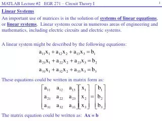
MATLAB Lecture #2 EGR 271 – Circuit Theory I. Linear Systems An important use of matrices is in the solution of systems of linear equations , or linear systems . Linear systems occur in numerous areas of engineering and mathematics, including electric circuits and electric systems.

Linear Systems
E N D
Presentation Transcript
MATLAB Lecture #2 EGR 271 – Circuit Theory I Linear Systems An important use of matrices is in the solution of systems of linear equations, or linear systems. Linear systems occur in numerous areas of engineering and mathematics, including electric circuits and electric systems. A linear system might be described by the following equations: These equations could be written in matrix form as: The matrix equation could be written as: Ax = b
MATLAB Lecture #2 EGR 271 – Circuit Theory I • Several methods can be used to solve linear systems in the form Ax = b, including: • Using the inverse matrix, A-1 • Gaussian elimination • Gauss-Jordan reduction
MATLAB Lecture #2 EGR 271 – Circuit Theory I Solving Linear Systems using A-1: Recall that when multiplying matrices that AB BA. As a result, if both sides of a matrix equation are multiplied by another matrix, there is a difference between pre-multiplying and post-multiplying. Example: B = C (original equation) AB = AC (pre-multiplying the original equation by matrix A) BA = CA(post-multiplying the original equation by matrix A) But since AB BA, the result of pre-multiplying and post-multiplying is clearly different. This needs to be kept in mind when solving linear equations in the form Ax = b. Ax = b (system of linear equations) A-1Ax = A-1b (pre-multiply by A-1) Ix = A-1b (since A-1A = I) x = A-1b (since Ix = x) So linear systems can be solved using x = A-1b x = inv(A)*b in MATLAB
MATLAB Lecture #2 EGR 271 – Circuit Theory I Example: Solve the system of equations below using x = A-1b with MATLAB. Solution: Note: MATLAB may give warnings about using this method to solve equations and may recommend a different method. We will discuss this later.
MATLAB Lecture #2 EGR 271 – Circuit Theory I Gaussian Elimination Which system of equations below is easier to solve? • The system on the right is easier because we can easily: • Solve for z in the 3rd equation • Substitute the value of z into the 2nd equation and solve for y • Substitute the values of y and z into the 1st equation and solve for x • The right set of equations is easier to solve for because it is in row-echelon form where we can easily use back substitution. • It may be hard to recognize, but the two systems of equations are equivalent!
MATLAB Lecture #2 EGR 271 – Circuit Theory I Gaussian Elimination Original equations Equations in row-echelon form Original equations in augmented matrixform Augmented matrix manipulated into row-echelon form The matrix was manipulated using elementary row operations. The process is called Gaussian elimination.
MATLAB Lecture #2 EGR 271 – Circuit Theory I Manipulating augmented matrices is similar to how we manipulate equations. Example: Example: Multiply both sides of an equation by 2 This was a type of elementary row operation Add 2 times Eq 1 to Eq 2 to form a new equation This was another type of elementary row operation. Note that Eq 2 was replaced by the new equation.
MATLAB Lecture #2 EGR 271 – Circuit Theory I • Elementary Row Operations • There are three types of elementary row operations: • Multiply a row by a non-zero constant • Notation: 3R1 (multiply row 1 by 3) • Interchange two rows • Notation: R2,3 (interchange row 2 and row 3) • Add a multiple of one row to another row • Notation: R2 + (3)R1 (add 3 times row 1 to row 2) • Note: Elementary column operations cannot be used to solve systems of equations, but they could perhaps be used in other applications not covered in this course.
MATLAB Lecture #2 EGR 271 – Circuit Theory I Example 1: Solve the following three equations using Gaussian elimination. Solution: Form the augmented matrix: Perform elementary row operations using column 1 as the pivot column: Perform elementary row operations using column 2 as the pivot column: Back substitute to solve for x, y, and z. Pivot element Pivot column The matrix is now in row-echelon form
MATLAB Lecture #2 EGR 271 – Circuit Theory I Note: Although it is not required, it is common to adjust each column so that the leading coefficient is 1. For the last example, we could continue as follows: Now the back substitution is even easier: Checking results: It is a good idea to check your results by substituting the answers back into the original equations. Try this for the problem above:
MATLAB Lecture #2 EGR 271 – Circuit Theory I Rearranging rows: When performing Gaussian reduction, the pivot element must be non-zero. If there is a zero in the pivot element position, it is useful to rearrange the rows (one of the three elementary row operations). Example: Solve the following system of equations.
MATLAB Lecture #2 EGR 271 – Circuit Theory I Gauss-Jordan Elimination: In using Gauss-Jordan elimination (or Gauss-Jordan reduction), we continue where Gaussian elimination left off and use additional elementary row operations until the augmented matrix is in reduced row-echelon form. This will eliminate the need for back substitution. Elementary row operations Elementary row operations Gaussian elimination Gauss-Jordan elimination Row-echelon form Use back substitution to find results Reduced row-echelon form Read results directly: x = 1, y = -1, z = 2 See next slide for step-by-step details
MATLAB Lecture #2 EGR 271 – Circuit Theory I Gauss-Jordan Elimination: Solve the system of equations below using Gauss-Jordan reduction (same example as on previous slide but detail added). Row-echelon form Solution: Reduced row-echelon form Pivot element Pivot column Results: x = 1, y = -1, z = 2
MATLAB Lecture #2 EGR 271 – Circuit Theory I Example: Solve the system of equations below using Gauss-Jordan reduction. Results: x = 3, y = -2, z = 4
MATLAB Lecture #2 EGR 271 – Circuit Theory I rref( ) - a useful function in MATLAB for reducing an augmented matrix into reduced row echelon form Example: Use rref( ) to solve the following systems of equations (both from earlier examples). System 2: System 1:
MATLAB Lecture #2 EGR 271 – Circuit Theory I Left Division in MATLAB - It is recommended that a system of linear equations in the form Ax = b be solved using left division x = A\b instead of using x = inv(A)*b • Advantage of using left division • In general, x = A\b is more stable and faster. Why? Some reasons include: • inv(A) may not exist • x = A\b uses Gaussian elimination and: • Scales matrix entries to minimize errors • Uses faster algorithms for special matrices, such as sparse, symmetrical or banded matrices.
MATLAB Lecture #2 EGR 271 – Circuit Theory I Example: - The following represents an ill-conditioned linear system. The error in the result depends highly on the number of significant digits used unless the equations are scaled. • Note the warning associated with using x1 = inv(A)*b. • Note that the results are different.
MATLAB Lecture #2 EGR 271 – Circuit Theory I • Example: A) Solve the following equations using Gauss-Jordan reduction • Solve the equations in MATLAB using three methods: • x = inv(A)*b • rref( ) • x = A\b KVL, meshes 1-3 yields: