Download

1 / 23
230 likes | 354 Vues
Competitive Industry in the Short Run. operating rule case 1. $/unit. MC. AC. The firm is a price taker - say it takes P. P. MR. a. b. AVC. This firm should operate where MR = MC and make a positive profit. c. Q or units. Q1. If firm operates if it shuts down

E N D
operating rule case 1 $/unit MC AC The firm is a price taker - say it takes P P MR a b AVC This firm should operate where MR = MC and make a positive profit c Q or units Q1 If firm operates if it shuts down TR = a + b + c TR = 0 TC = b + c TC = TFC = b profit = a profit = -b.
Profit I copied the slide form a previous set of notes. Recall we said the firm should produce the Q where MR = MC and have profit = (P – AC)Q. Well PROFIT = TR – TC = P(Q) – TC(Q/Q) = (P – (TC/Q))Q = (P – AC)Q. At the Q in the graph on the previous screen rectangle a has area (P – AC)Q. This is the profit amount.
We said the short run is the period of time in which at least one input is fixed. In the industry this means the number of firms is also fixed – firms outside the industry also can not get more of some input and since they are not in the industry they can not join it in the short run. Since each firm’s supply curve is its MC curve above the AVC, the industry supply is the sum of each firm’s MC. We call the industry supply the horizontal sum of each firms supply because in the graph we sum the q’s of each firm at each price. Let’s see this on the next screen.
P Here we just have two firms. If more, follow the same principle. Many times we just show a smooth upward sloping curve just to show the basic idea. Firm 1 Add firm 1 onto firm 2 Firm 2 Q
Say you have a competitive market where the demand for consumers has been added up to be Qd = 6000/9 – (50/9)P. Also say there are 50 identical firms, where each has the total cost TC = 100 + 10Q + Q2. The marginal cost for each firm would be MC = 10 + 2Q. We know that firms that maximize profit produce the level of output where MR = MC (as long as P>=AVC). For a competitive firm P = MR, so MR = MC means P = 10 + 2Q, or Q = (P – 10)/2 = .5P – 5 for each firm.
We know the supply curve in the competitive industry is basically the summation of the MC of each firm in the industry. For one firm we have in our example P = 10 + 2Q. To add across all 50 firms we re-express MC as Q = .5P – (10/2). Now we add all 50 firms together: Q = .5P – (10/2) Q = .5P – (10/2) (if firms are not identical, follow this … same basic process.) Q = .5P – (10/2) Qs = 25P – 250 or P = 1/25Q + 10 The supply curve
Note the supply curve, Qs, adds up the supply curve of each firm. .5P 50 times is 25P and (10/2) 50 times is 250. So for the supply curve we have Qs = 25P – 250. The market price and quantity traded are determined where Qs = Qd, so we have 25P – 250 = 6000/9 – (50/9)P, or (225/9)P + (50/9)P = 6000/9 + 2250/9, or (275/9)P = 8250/9, or P = 8250/275 = 30. Plug P = 30 into either Qd or Qs to get the quantity traded in the market. In Qs we have 25(30) – 250 = 500.
Since the market price is 30, each firm will make Q= (P – 10)/2 = (30-10)/2 = 10. The profit for each firm TR – TC. TR for a firm is P times Q, or PQ. TR = 30(10) = 300. TC = 100 + 10Q + Q2 for each firm in this example. So, TC = 100 + 10(10) + 102 = 300. Profit = 300 – 300 = 0.
P D1 S1 ATC1 MC1 P1 =30 P=MR1 Q q Q1=500 Q1=10 Market Firm
Here we have the industry P and Q where S=D and the firm output level q where MR = MC, or we could say P = MC since P=MR. (presumably the firms MC are above AVC, so we have profit max positions.) P S MC = S P=D =MR = AR D Q Industry or market firm
Change in fixed cost A change in the fixed cost for firms in the industry will not change the industry at all in the short run. In the short run a change in fixed cost will just affect the amount of profit for the firm. But it can not drive the firm out since the MC is above the AVC. Variable costs are covered and some amount of the fixed cost has to be covered. In the long run we could have a very different story. But, let’s look at an analogy to get the short run story. The fish tank analogy. Look at the next several slides quickly, to simulate a fish tank being filled with water.
Hose and water going into tank Water level
Hose and water going into tank Water level
Hose and water going into tank Water level
Hose and water going into tank Water level
Wow, this is wild! Hose and water going into tank Water level
Here is where we get the pay – off from the fish bowl analogy. Given the price, the firm looks at its revenue as e and f filling the tank as shown by d+e+f. Have the water fill in from the bottom up. Since the revenue covers the TVC – area f - and some of the TFC – area d + e – it is better to operate. A change in the fixed cost doesn’t change the fact that TVC would be covered and some of the fixed cost. If the firm shut down it would have no variable cost and all the fixed cost to pay with no revenue. By producing, the revenue covers all the variable and some of the fixed. So the firm loses less. $/unit MC AC d MR P e AVC f Q1 Q or units Remember, see the revenue fill area f and e from the bottom up.
Say variable costs rise in such a way that MC for firms rises. Here I show the MC curve shift left. The industry supply will shift left because the industry is simply the sum of all the firms. Market price will rise and output will fall. With a higher market price the firm demand line = price line will rise. Where I show the industry supply, the price means the firm would have the same level of output as before the change. Can this be? S MC = S P P=D =MR = AR D Q Industry or market firm
The output for all firms in the industry can not be the same if the output in the industry is lower. On average, output has to fall at the firm level. If the firm shown had had slightly steeper curves the output for the firm would have fallen. So, we see a special case in my graph. Demand in market rises If demand in the market rises we would see a higher price and a greater quantity coming out of the market. Each firm would have more output at the higher price. Next, we want to explore the cost of making the industry output. The conclusion is that firms as a group will make the industry output the cheapest that it can be made. Let’s turn to this next.
Refresher – What information the marginal cost curve contains. At a quantity, the height of the MC curve tells us how much is added to cost when that unit is added. The height would also tell us how much cost would go down if that unit was not produced. $ MC Q
The output made in the market is made with the lowest cost. Let’s see how. Normally each firm makes Q where MR = MC and since P = MR, P = MC. Say I have power to make firms change – say I make firm 1 make 1 more unit and to keep total output the same I make firm 2 make 1 less. Firm 1’s cost goes up by price + something. Firm 2’s cost goes down by the price. $ $ $ MC1 MC2 S P D Q Q Q Q1 Q2 Market – scale is larger than each firm Firm 1 Firm 2 So price + something minus price = something. Making firms change from what they want makes cost of market output rise.