Equilibrium Output in the Short-Run

1. Equilibrium Output in the Short-Run Antu Panini Murshid

2. Today’s Agenda • The components and determinants of aggregate demand in an open economy • Goods market equilibrium • Asset market equilibrium • Short run equilibrium in an open economy

3. Components of Aggregate Demand • It is useful to decompose aggregate demand into four components: • Consumption spending • Planned investment • Government spending • Net exports

4. Determinants of Consumption • Disposable income • Income minus taxes (Y-T) • Permanent income • Real wealth • Real interest rate Typically we will assume that taxes are lump sum

5. Consumption Function • Since consumption is a function of disposable income we can write C = C(Yd,a), where Yd≡ Y-T, and a denotes all other arguments • A linear consumption function would take the following form: C = a + bYd Autonomous consumption Marginal propensity to consume

6. Autonomous Consumption • Autonomous consumption is that part of consumption which is not effected by disposable income • These are expenditures that would occur even if household disposable income was zero • What determines autonomous consumption? • Other determinants of consumption, e.g. wealth, real interest rates, etc.

7. Marginal Propensity to Consume • The proportion of each additional dollar of income that is used for consumption expenditures • The marginal propensity to consume is just the slope of the consumption function

8. Marginal Propensity to Consume • Normally we assume that the MPC is less than one • Why is this a reasonable assumption? • Because some proportion of each additional dollar of income is devoted to savings

9. A Linear Consumption Function Against Yd • Autonomous consumption is just the intercept • Note the slope of the consumption function is less than one consumption 450 c = a + b(Y-T) • Note also that the consumption function is drawn against disposable income • What would the consumption function look like, if we drew it against income? autonomous consumption slope = marginal propensity to Consume (b) a disposable income (Y-T)

10. A Linear Consumption Function Against Y • If we draw consumption against income, the intercept becomes (a-bT1) consumption 450 c = a + b(Y-T1) c = a + b(Y-T2) • What happens to the consumption function if we increase taxes? • The consumption function shifts downward a-bT1 a-bT2 income (Y)

11. Determinants of Planned Investment • Real interest rate (cost of borrowing) • Rate of return on capital (marginal product of capital) • Risk and future expectations

12. A Linear Investment Schedule real interest rate 2…planned investment increases 5% 4% 1. As the real interest rate falls… Planned investment 1,000 1,500 Investment

13. Shifts in the Investment Schedule An increase in the return to investments shifts the schedule to the right real interest rate A decline in the riskiness of investments has the same effect 5% I2 I1 1,000 1,500 Investment

14. First draw the consumption function Now add investment Adding Up Consumption and Investment 450 consumption C + I1 = a + b(Y-T) + I1 C = a + b(Y-T) Investment a-bT income (Y)

15. Impact of an Increase in Investment • A reduction in the interest rate, change in expectations, etc. will raise investment and shift C+I schedule up 450 consumption C + I2 C + I1 income (Y)

16. Assumption: Planned Investment is Exogenous • While there are several determinants of planned investment, let us assume that it is exogenously given • This will make life simpler and let us focus on other important channels by which income is affected in an open economy

17. Assumption: Government Savings • As with planned investment, let us assume that government spending is exogenously given • Again this is a simplification that lets us focus on the important open-economy channels that impact on income

18. What About Net Exports? • One component of expenditure that we cannot simply treat as exogenous is net exports • Net exports have an important influence on aggregate demand in open economies and one that distinguishes it from closed economies • Below we consider the determinants of exports and imports separately

19. Determinants of Exports • World income • An increase in world income, increases the demand for exports • Real exchange rates • A depreciation in the real exchange rate makes domestically produced goods more competitive and so increases the demand for our exports

20. Determinants of Imports • Domestic income • An increase in domestic disposable income will increase the demand for imports • Real exchange rates • A depreciation in the real exchange rate will have an ambiguous effect on imports • Why?

21. Real Exchange Rate and Imports • There are two effects that a real exchange rate depreciation will have: • Lower the volume of imports • Increase the price of imports • There are therefore opposing forces at work since the total value of imports is just: Value of imports = price * volume ?

22. The Marshall-Lerner Condition • So what will be the overall effect of a real exchange rate depreciation on net exports? • The Marshall-Lerner condition says that a real exchange rate depreciation will improve the trade balance if: ηx+ηM>1, where ηX is the elasticity of demand for exports and ηM is the elasticity of demand for imports • Can you prove this (assume NX = 0)?

23. If demand is inelastic a reduction an exchange rate depreciation and a rise in the price of imports has little impact on quantity of imports demanded, hence value of imports rises: If demand is elastic the same change in price has a much larger impact on volumes and so imports fall Intuition Behind the M-L Condition: Elasticity of Imports price of imports Increase in imports Decrease in imports p2 p1 D2 D1 Q2 q2 q1 Q1 quantity of exports

24. When export-demand is elastic an exchange rate depreciation which lowers the foreign price of exports, has a large impact on the quantity demanded This implies that the value of exports necessarily rises significantly since the domestic price received for exports has not changed Intuition Behind the M-L Condition: Elasticity of Exports foreign price of exports Large increase in exports demand pf1 pf2 D Q1 Q2 quantity of exports

25. Does the Marshall-Lerner Condition Hold? The J-Curve • In our analysis, we will assume that the Marshall-Lerner condition holds • Is this a good assumption? • Yes and no • Often the initial effect of a depreciation is to cause the trade deficit to increase, over time however the deficit improves. This is known as the J-curve effect

26. Reasons for the J-Curve • Import and export volumes are slow to adjust after exchange rate changes • Most import and export orders are placed months in advance, hence the primary effect of a depreciation is to raise the value of the pre-contracted level of imports

27. Summarizing the Determinants of AD: Income • ↑ disposable income ⇒ • ↑ consumption + ↑ imports • Net effect ↑ aggregate demand • Why? Why does the increase in import demands not dominate the increase in consumption

28. Summarizing the Determinants of AD: World Income • ↑ world income ⇒ • ↑ exports • Net effect ↑ aggregate demand

29. Summarizing the Determinants of AD: Real Exchange Rate • We will assume that the Marshall-Lerner condition holds • ↑ θ (real ex depreciation) ⇒ • Note ↑ θ (real ex depreciation) implies either • ↑ e (nominal exchange rate) • ↑ Pf (foreign price level) • ↓ P (domestic price level) • ↑ exports + ↓ imports • Net effect ↑ aggregate demand All of these factors will increase θ

30. Summarizing the Determinants of AD: Other Determinants • There are several other determinants of AD • real interest rate, productivity of capital, future expectations, etc. • However in the analysis below we focus on the impact of disposable income and the real exchange rate on consumption and net exports, all other variables are treated as exogenous

31. Equation For Aggregate Demand AD = C(Yd) + I + G + NX(θ,Yd,Y*)

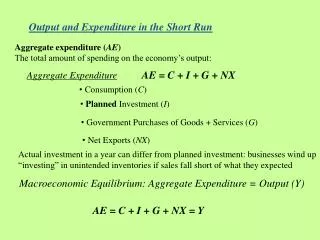
32. Aggregate Demand Function 450 consumption C + I +G Government spending C + I +G + NX=aggregate expenditures C + I Net exports C=f(Y) • Consumption + • Investment + • Government spending + • Net exports = • Planned aggregate expenditures • Note in this example net exports are negative Investment income (Y)

33. Slope of Aggregate Demand Function in Open Economy • Note that the slope of the aggregate demand function is less than the slope of the domestic absorption function. Why? • Because imports increase with income • The proportion of each additional dollar of household income that is used for imports is called the marginal propensity to import (MPM) • The slope of the aggregate demand function is equal to MPC-MPM

34. The following factors will increase aggregate demand: ↓ taxes, ↑ government spending, ↑ planned investment, ↑ θ, ↑ world incomes, ↑ autonomous consumption a shift in preferences for domestic goods over foreign goods Illustrating Increases in Aggregate Demand 450 aggregate expenditures AD2 AD1 ↑ AD income (Y)

35. Quick Quiz • Can you illustrate the impact of the following on aggregate demand: • An exchange rate depreciation • A decline in the foreign price level • A fall in world real income • A rise in lump sum taxes

36. Goods Market Equilibrium • What is the equilibrium level of income in an economy? • We would like to have some notion of equilibrium where the demand for goods and services is equal to the supply. Therefore we define an equilibrium in the goods markets as follows: Total Output Produced = Planned AE (AD) Y = C + I + G + NX

37. Goods Market Equilibrium: Graphical Illustration 450 aggregate expenditures C + I +G + NX=aggregate expenditures C=f(Y) • At every point on the 450 line, income = aggregate expenditures • Hence the equilibrium is where the planned aggregate expenditures intersects the 450 line Y* income (Y)

38. Initially suppose equilibrium income is Y1 Now suppose net exports rise (for whatever reason), then AD rises and so too does equilibrium income Impact of an Increase in Net Exports on Equilibrium Output 450 aggregate expenditures AD2 AD1 ↑ AD Y1 Y2 income (Y)

39. Aggregate Demand, Output and Exchange Rates • Is aggregate demand and income related to the exchange rate? • Clearly yes. What is this relationship? • If the M-L condition holds we know that an increase in θ increases AD • Hence all else equal an increase in the nominal exchange rate should imply an increase in AD. This will imply an increase in equilibrium income/output

40. Recap on the Intuition • When the nominal exchange rate rises (depreciates), all else equal: • Exports become more competitive and thus exports increase • If the M-L condition holds imports will decline because imports are now more expensive • Hence AD increases • This in turn implies an increase in income

41. The DD-Schedule • The DD-schedule illustrates the relationship between the nominal exchange rate and the level of income or output such that the goods market is in equilibrium • The DD-schedule must be positively sloped since an increase in the nominal exchange rate implies an increase in equilibrium output

42. Equilibrium income is Y1 suppose the exchange rate is e1 Now suppose the exchange rate rises to e2 AD ↑ and Y ↑ to Y2 Hence the new exchange rate-income combination is e2,Y2 The locus of such points traces out the DD-curve Deriving the DD Schedule AD2 Aggregate expenditures AD1 income Exchange rate Y1 Y2 DD e2 e1 income Y1 Y2

43. Shifts in the DD-Schedule • What would shift the DD-schedule? • Anything other than a change in the nominal exchange rate, which affects the equilibrium level of income • Examples • A change in fiscal policy • A change in planned investment • A change in the domestic or foreign price level • A change in autonomous consumption • A change in the preferences for domestic goods over foreign goods

44. Quick Quiz • Which way will the DD-curve shift if: • planned investment rises • domestic price level rises • consumers express an increased preference for foreign goods

45. Asset Markets • So far our analysis has focused on the goods market. Now we will introduce asset markets • We will assume that there are only two markets • Money market • Foreign exchange market

46. Asset Markets Equilibrium • The money market is in equilibrium if: demand for money = supply of money P*L(y,i) = Ms • The foreign-exchange market is in equilibrium if: domestic interest rate = expected return on foreign assets i = if + E(%∆e)

47. What is Determined in Asset Markets? • What is determined in the money market? • Equilibrium interest rate • What is determined in the foreign exchange market? • Equilibrium exchange rate

48. We have already discussed the relationship between the exchange rate and the interest rate, but lets take another look First draw the money market graph The equilibrium interest rate is 10% Exchange Rate and the Interest Rate Money supply M1s/P Interest rate Equilibrium interest rate i1=10% Money demand L(i,y) real money balances

49. Now lets make everything disappear…. Exchange Rate and the Interest Rate Money supply M1s/P Interest rate Equilibrium interest rate i1=10% Money demand L(i,y) real money balances

50. …and reappear but rotated clockwise by 90 degrees Exchange Rate and the Interest Rate i1=10% Interest rate Money supply M1s/P Equilibrium interest rate real money balances Money demand L(i,y)