Download
1 / 32
320 likes | 449 Vues
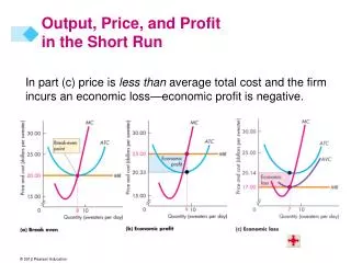
Output, Price, and Profit in the Short Run. In part (c) price is less than average total cost and the firm incurs an economic loss—economic profit is negative. Output, Price, and Profit in the Long Run.

E N D
Output, Price, and Profit in the Short Run In part (c) price is less than average total cost and the firm incurs an economic loss—economic profit is negative.
Output, Price, and Profit in the Long Run In short-run equilibrium, a firm might make an economic profit, break even, or incur an economic loss. Only one of them is a long-run equilibrium because firms can enter or exit the market.
Output, Price, and Profit in the Long Run Entry and Exit New firms enter an industry in which existing firms make an economic profit. Firms exit an industry in which they incur an economic loss. Figure 12.9 shows the effects of entry and exit.
Output, Price, and Profit in the Long Run A Closer Look at Entry When the market price is $25 a sweater, firms in the market are making economic profit.
Output, Price, and Profit in the Long Run New firms have an incentive to enter the market. When they do, the market supply increases and the market price falls.
Output, Price, and Profit in the Long Run Firms enter as long as firms are making economic profits. In the long run, the market price falls until firms are making zero economic profit.
Output, Price, and Profit in the Long Run A Closer Look at Exit When the market price is $17 a sweater, firms in the market are incurring economic loss.
Output, Price, and Profit in the Long Run Firms have an incentive to exit the market. When they do, the market supply decreases and the market price rises.
Output, Price, and Profit in the Long Run Firms exit as long as firms are incurring economic losses. In the long run, the price continues to rise until firms make zero economic profit.
Changing Tastes and Advancing Technology A Permanent Change in Demand A decrease in demand shifts the market demand curve leftward. The price falls and the quantity decreases. Starting from long-run equilibrium, firms incur economic losses. Figure 12.10 illustrates the effects of a permanent decrease in demand.
Changing Tastes and Advancing Technology The market demand curve leftward, the market price falls, and each firm decreases the quantity it produces.
Changing Tastes and Advancing Technology The market price is now below each firm’s minimum average total cost, so firms incur economic losses.
Changing Tastes and Advancing Technology Economic losses induce some firms to exit in the long run, which decreases the market supply and the price starts to rise.
Changing Tastes and Advancing Technology As the price rises, the quantity produced by all firms continues to decrease as more firms exit, but each firm remaining in the market starts to increase its quantity.
Changing Tastes and Advancing Technology A new long-run equilibrium occurs when the price has risen to equal minimum average total cost. Firms make zero economic profits, and firms no longer exit the market.
Changing Tastes and Advancing Technology The main difference between the initial and new long-run equilibrium is the number of firms in the market. Fewer firms produce the equilibrium quantity.
Changing Tastes and Advancing Technology A permanent increase in demand has the opposite effects to those just described and shown in Figure 12.10. A permanent increase in demand shifts the demand curve rightward. The price rises and the quantity increases. Economic profit induces entry, which increases short-run supply and shifts the short-run market supply curve rightward. As the market supply increases, the price falls and the market quantity continues to increase.
Changing Tastes and Advancing Technology With a falling price, each firm decreases its output as it moves along its marginal cost curve (supply curve). A new long-run equilibrium occurs when the price has fallen to equal minimum average total cost. Firms make zero economic profit, and firms have no incentive to enter the market. The main difference between the initial and new long-run equilibrium is the number of firms. In the new equilibrium, a larger number of firms produce the equilibrium quantity.
Changing Tastes and Advancing Technology External Economics and Diseconomies The change in the long-run equilibrium price following a permanent change in demand depends on external economies and external diseconomies. External economies are factors beyond the control of an individual firm that lower the firm’s costs as the industry output increases. External diseconomies are factors beyond the control of a firm that raise the firm’s costs as industry output increases.
Changing Tastes and Advancing Technology In the absence of external economies or external diseconomies, a firm’s costs remain constant as the market output changes. Figure 12.11 illustrates the three possible cases and shows the long-run market supply curve. The long-run market supply curve shows how the quantity supplied in a market varies as the market price varies after all the possible adjustments have been made, including changes in each firm’s plant and the number of firms in the market.
Changing Tastes and Advancing Technology Figure 12.11(a) shows that in the absence of external economies or external diseconomies, an increase in demand does not change the price in the long run. The long-run market supply curve LSA is horizontal.
Changing Tastes and Advancing Technology Figure 12.11(b) shows that when external diseconomies are present, an increase in demand brings a higher price in the long run. The long-run market supply curve LSB is upward sloping.
Changing Tastes and Advancing Technology Figure 12.11(c) shows that when external economies are present, an increase in demand brings a lower price in the long run. The long-run market supply curve LSC is downward sloping.
Changing Tastes and Advancing Technology Technological Change New technologies are constantly discovered that lower costs. A new technology enables firms to produce at a lower average cost and a lower marginal cost—firms’ cost curves shift downward. Firms that adopt the new technology make an economic profit.
Changing Tastes and Advancing Technology New-technology firms enter and old-technology firms either exit or adopt the new technology. Industry supply increases and the industry supply curve shifts rightward. The price falls and the quantity increases. Eventually, a new long-run equilibrium emerges in which all firms use the new technology, the price equals minimum average total cost, and each firm makes zero economic profit.
Competition and Efficiency Efficient Use of Resources Resources are used efficiently when no one can be made better off without making someone else worse off. This situation arises when marginal social benefit equals marginal social cost.
Competition and Efficiency Choices, Equilibrium, and Efficiency We can describe an efficient use of resources in terms of the choices of consumers and firms coordinated in market equilibrium. Choices A consumer’s demand curve shows how the best budget allocation changes as the price of a good changes. So consumers get the most value out of their resources at all points along their demand curves. With no external benefits, the market demand curve is the marginal social benefit curve.
Competition and Efficiency A competitive firm’s supply curve shows how the profit-maximizing quantity changes as the price of a good changes. So firms get the most value out of their resources at all points along their supply curves. With no external cost, the market supply curve is the marginal social cost curve.
Competition and Efficiency Equilibrium and Efficiency In competitive equilibrium, resources are used efficiently—the quantity demanded equals the quantity supplied, so marginal social benefit equals marginal social cost. The gains from trade for consumers is measured by consumer surplus. The gains from trade for producers is measured by producer surplus. Total gains from trade equal total surplus.In long-run equilibrium total surplus is maximized.
Competition and Efficiency Figure 12.12 illustrates an efficient allocation of resources in a perfectly competitive market. At the market price P*, each firm is producing the quantity q*at the lowest possible long-run average total cost.
Competition and Efficiency Figure 12.12(b) shows the market. Along the market demand curve D = MSB, consumers are efficient. Along the market supply curve S = MSC, producers are efficient.
Competition and Efficiency The quantity Q* and price P* are the competitive equilibrium values. So competitive equilibrium is efficient. Total surplus, the sum of consumer surplus and producer surplus, is maximized.