Download
1 / 72
720 likes | 896 Vues
Spending and Output in the Short Run. Introduction. Observations Spending, in the short run, may not be sufficient to support a normal level of output. Therefore, recessionary gaps are caused by insufficient aggregate spending. Introduction. John Maynard Keynes

E N D
Spending and Output in the Short Run
Introduction • Observations • Spending, in the short run, may not be sufficient to support a normal level of output. • Therefore, recessionary gaps are caused by insufficient aggregate spending. Chapter 13: Spending and Output in the Short Run
Introduction • John Maynard Keynes • Economist, diplomat, financier, journalist, and patron of the arts • Publications include: • The Economic Consequences of the Peace • The General Theory of Employment, Interest, and Money Chapter 13: Spending and Output in the Short Run
Introduction • John Maynard Keynes • The General Theory: • Revolutionized economic policy • Predicted that a decrease in aggregate spending could create a recessionary gap • Suggests that government policy could be used to restore full employment Chapter 13: Spending and Output in the Short Run
The Keynesian Model’s Crucial Assumption: Firms Meet Demand at Preset Prices • In the short run, firms meet the demand for their products at preset prices. • Firms do not respond to every change in the demand for their products by changing their prices. • Instead, they typically set a price for some period, then meet the demand at that price. Chapter 13: Spending and Output in the Short Run
The Keynesian Model’s Crucial Assumption: Firms Meet Demand at Preset Prices • In the short run, firms meet the demand for their products at preset prices. • By “meeting the demand,” we mean that firms produce just enough to satisfy their customers at the prices that have been set. Chapter 13: Spending and Output in the Short Run
The Keynesian Model’s Crucial Assumption: Firms Meet Demand at Preset Prices • Meeting Demand at Preset Prices: • Is a logical management decision because of menu costs. • Menu costs – the costs of changing prices • Prices should be changed only if the benefit exceeds the menu cost. • In the long run firms will change prices. Chapter 13: Spending and Output in the Short Run
The Keynesian Model’s Crucial Assumption: Firms Meet Demand at Preset Prices • Economic Naturalist • Will new technologies eliminate menu costs? • Keynesian theory assumes that menu cost prevent firms from changing prices. • Many new technologies (bar codes) have reduced menu cost and increased price flexibility. Chapter 13: Spending and Output in the Short Run
The Keynesian Model’s Crucial Assumption: Firms Meet Demand at Preset Prices • Economic Naturalist • Will new technologies eliminate menu costs? • Pricing decisions also require market analysis, strategic considerations, and cost analysis. • These factors are a component of menu costs. Chapter 13: Spending and Output in the Short Run
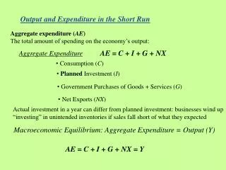
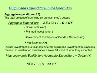
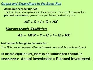
Planned Aggregate Expenditure • Planned Aggregate Expenditure • Total planned spending on final goods and services Chapter 13: Spending and Output in the Short Run
Planned Aggregate Expenditure • The Components of Planned Aggregate Expenditure • Consumer expenditure or Consumption (C) • Household spending on durables, nondurables, and services Chapter 13: Spending and Output in the Short Run
Planned Aggregate Expenditure • The Components of Planned Aggregate Expenditure • Investment (I) • New capital goods spending • New residential spending • Increases in inventories Chapter 13: Spending and Output in the Short Run
Planned Aggregate Expenditure • The Components of Planned Aggregate Expenditure • Government purchases • Federal, state, and local spending on goods and services Chapter 13: Spending and Output in the Short Run
Planned Aggregate Expenditure • The Components of Planned Aggregate Expenditure • Net exports • Exports - Imports Chapter 13: Spending and Output in the Short Run
Planned Aggregate Expenditure • Planned Spending Versus Actual Spending • In the Keynesian model, output is determined by PAE. • Actual expenditures may not equal PAE. • If inventories are larger than expected: • I > planned investment (IP) • If inventories are smaller than expected: • I < IP Chapter 13: Spending and Output in the Short Run
Planned Aggregate Expenditure • Example • Actual and planned investment • Fly-by-Night Kite Co. produces $5 million of kites per year. • Expected sales = $4.8 million and planned inventory = $200,000 • Capital expenditure = $1 million Chapter 13: Spending and Output in the Short Run
Planned Aggregate Expenditure • Example • If actual sales are: • $4,600,000 instead of $4,800,000 • IP = $1,000,000 + $200,000 = $1,200,000 • I = $1,200,000 + $200,000 = $1,400,000 • I > IP • $4,800,000 • IP = $1.2 m. = I Chapter 13: Spending and Output in the Short Run
Planned Aggregate Expenditure • Example • If actual sales are: • $5,000,000 • IP = $1,000,000 + $200,000 = $1,200,000 • I = $1,200,000 - $200,000 = $1,000,000 • I < IP Chapter 13: Spending and Output in the Short Run
Planned Aggregate Expenditure • Planned Aggregate Expenditure Chapter 13: Spending and Output in the Short Run
Planned Aggregate Expenditure • Hey Big Spender! Consumer Spending and the Economy • Consumption (C) accounts for two thirds of total spending • The primary determinant of C is disposable income or Y - T Chapter 13: Spending and Output in the Short Run
Planned Aggregate Expenditure • Consumption Function • The relationship between consumption spending and its determinants, in particular, disposable (after-tax) income Chapter 13: Spending and Output in the Short Run
Planned Aggregate Expenditure • Relating Consumption to Income and Other Determinants • The consumption function: • C = a constant; represents the non income determinants of C • Consumer optimism • Wealth • Real interest rates Chapter 13: Spending and Output in the Short Run
Planned Aggregate Expenditure • Economic Naturalist • What effect did the 2000-2002 decline in the U.S. stock market values have on consumption spending? • From March 2000 to March 2002 the S&P 500 fell 49%. • Households lost $6.5 trillion of wealth in two years Chapter 13: Spending and Output in the Short Run
Planned Aggregate Expenditure • Economic Naturalist • What effect did the 2000-2002 decline in the U.S. stock market values have on consumption spending? • $1 decrease in wealth reduces C by 3 to 7 cents/year • The $6.5 trillion loss could reduce C between $195 and $455 billion Chapter 13: Spending and Output in the Short Run
Planned Aggregate Expenditure • Economic Naturalist • What effect did the 2000-2002 decline in the U.S. stock market values have on consumption spending? • C rose from 2000-2002 • Higher housing prices (greater wealth) • Lower interest rates • Increase in disposable income (Y – T) Chapter 13: Spending and Output in the Short Run
Planned Aggregate Expenditure • Consumption Function • mpc = marginal propensity to consume • mpc = the amount by which consumption rises when disposable income rises by $1; 0 < mpc < 1 Chapter 13: Spending and Output in the Short Run
Consumption function Slope = mpc C A Consumption Function Consumption spending C Disposable income Y-T Chapter 13: Spending and Output in the Short Run
The U.S. Consumption Function, 1960-2004 Chapter 13: Spending and Output in the Short Run
Planned Aggregate Expenditure • Planned Aggregate Expenditure and Output • The relationship between changes in production and income and PAE • C is a large part of PAE • C depends on Y • PAE depends on Y Chapter 13: Spending and Output in the Short Run
Planned Aggregate Expenditure • Example • PAE = C + IP + G + NX • C = C + mpc(Y – T) • PAE = C + mpc(Y – T) + IP + G + NX • C = 620; mpc = 0.8; T = 250; IP= 220; G = 330; NX = 20 Chapter 13: Spending and Output in the Short Run
Planned Aggregate Expenditure • Example • Then: Chapter 13: Spending and Output in the Short Run
Planned Aggregate Expenditure • Example • If Y increases by $1, C will increase by 80 cents (mpc = 0.80) • C is part of PAE • PAE increases by 80 cents ($1 X 0.80) Chapter 13: Spending and Output in the Short Run
Planned Aggregate Expenditure • Example • There are two parts to PAE: • Autonomous expenditure (960) • Is independent of output • Does not vary when output changes • Induced expenditure (0.8Y) • Depends on output (Y) Chapter 13: Spending and Output in the Short Run
Planned Aggregate Expenditure • Example • PAE = autonomous expenditure + induced expenditure Chapter 13: Spending and Output in the Short Run
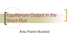
Planned Aggregate Expenditure • Short-run Equilibrium Output • The level of output at which output Y equals planned aggregate expenditure PAE • The level of output that prevails during the period in which prices are predetermined Chapter 13: Spending and Output in the Short Run
Planned Aggregate Expenditure • Short-run Equilibrium Output • Keynesian Assumption • Producers meet demand at preset prices in the short-run • Short-run equilibrium: Y = PAE Chapter 13: Spending and Output in the Short Run
Planned Aggregate Expenditure • Short-run Equilibrium Output • Three ways to find short-run equilibrium output: • Table to compute Y – PAE = 0 • The Keynesian Cross • Algebra Chapter 13: Spending and Output in the Short Run
(1) Output Y (2) Planned aggregate expenditure PAE = 960 + 0.8Y (3) Y - PAE (4) Y = PAE? 4,000 4,160 -160 No 4,200 4,320 -120 No 4,400 4,480 -80 No 4,600 4,640 -40 No 4,800 4,800 0 Yes 5,000 4,960 40 No 5,200 5,120 80 No Numerical Determination of Short-Run Equilibrium Output • Equilibrium: Y = PAE; Y (4,800) = PAE (4,800) • If Y = 4,000 < PAE = 960 + .8(4000) = 4,160 • If Y = 5,000 > PAE = 960 + .8(5,000) = 4,960 Chapter 13: Spending and Output in the Short Run
Y = PAE Expenditure line PAE = 960 + 0.8Y Slope = 0.8 • Equilibrium • PAE intersects the 45o line @ 4,800 • Disequilibrium • < 4,800, PAE > Y • > 4,800, PAE < Y 960 45o 4,800 Determination of Short-Run Equilibrium Output (Keynesian Cross) Planned aggregate expenditure PAE Output Y Chapter 13: Spending and Output in the Short Run
Y = PAE Expenditure line PAE = 960 + 0.8Y Slope = 0.8 • Equilibrium Algebraically • At equilibrium: PAE = C + Ip + G + NX • PAE = 960 + 0.8Y • 0.2Y = 960 • Y = 960/0.2 = 4,800 = equilibrium 960 45o 4,800 Determination of Short-Run Equilibrium Output (Keynesian Cross) Planned aggregate expenditure PAE Output Y Chapter 13: Spending and Output in the Short Run
Y = PAE Expenditure line PAE = 960 + 0.8Y Expenditure line PAE = 950 + 0.8Y E A decline in autonomous aggregate expenditure (C) shifts the expenditure line down F 960 950 Recessionary gap 45o 4,750 4,800 Y* A Decline In Planned Spending Leads to a Recession Planned aggregate expenditure PAE Output Y Chapter 13: Spending and Output in the Short Run
(1) Output Y (2) Planned aggregate expenditure PAE = 960 + 0.8Y (3) Y - PAE (4) Y – PAE? 4,600 4,630 -30 No 4,650 4,670 -20 No 4,700 4,710 -10 No 4,750 4,750 0 Yes 4,800 4,790 10 No 4,850 4,830 20 No 4,900 4,870 30 No 4,950 4,910 40 No 5,000 4,950 50 No Determination of Short-Run Equilibrium Output After a Fall In Spending • If Y = 4,800 > PAE = 4,790 • Y = PAE @ 4,750 • Output Gap: Y* (4,800) > Y (4,750) Chapter 13: Spending and Output in the Short Run
Planned Aggregate Expenditure • Observations • Other factors remaining constant, a decline in autonomous spending causes short-run equilibrium output to fall and creates a recessionary gap. • A decrease in autonomous spending can be caused by a reduction in C, IP, G, and/or NX. Chapter 13: Spending and Output in the Short Run
Planned Aggregate Expenditure • Economic Naturalist • Why was the deep Japanese recession of the 1990s bad news for the rest of East Asia? • Recession in Japan reduced Japanese imports • The decline in East Asian exports to Japan reduced domestic spending in non-export sectors Chapter 13: Spending and Output in the Short Run
Planned Aggregate Expenditure • Economic Naturalist • What caused the 2001 recession in the United States? • Reduction in investment spending Chapter 13: Spending and Output in the Short Run
Planned Aggregate Expenditure • Income-Expenditure Multiplier • The effect of a 1-unit increase in autonomous expenditure on short-run equilibrium output • For example, a multiplier of 5 means that a 10-unit decrease in autonomous expenditure reduces short-run equilibrium output by 50 units Chapter 13: Spending and Output in the Short Run
Planned Aggregate Expenditure • The Multiplier • Recall • PAE = 960 + 0.8Y, equilibrium Y = 4,800 • C fell by 10 • PAE = 950 + 0.8Y, equilibrium Y = 4,750 Chapter 13: Spending and Output in the Short Run
Planned Aggregate Expenditure • The Multiplier Effect • The decrease in the equilibrium Y was 5 times the fall in C. • The income-expenditure multiplier equaled 5. • The size of the multiplier is influenced by the mpc. Chapter 13: Spending and Output in the Short Run
Planned Aggregate Expenditure • What Do You Think? • Why is the change in equilibrium Y a multiple of the change in autonomous spending? Chapter 13: Spending and Output in the Short Run
Stabilizing Planned Spending: The Role of Fiscal Policy • In the Keynesian Model: • Recessionary and expansionary gaps are caused by inadequate or excessive spending, respectively. • Stabilization policies are used to affect planned aggregate expenditures to eliminate output gaps. Chapter 13: Spending and Output in the Short Run