Download

1 / 43
430 likes | 492 Vues
Markov-Chain Monte Carlo. CSE586 Computer Vision II Spring 2010, Penn State Univ. References. Recall: Sampling Motivation.

E N D
Markov-Chain Monte Carlo CSE586 Computer Vision II Spring 2010, Penn State Univ.
Recall: Sampling Motivation If we can generate random samples xi from a given distribution P(x), then we can estimate expected values of functions under this distribution by summation, rather than integration. That is, we can approximate: by first generating N i.i.d. samples from P(x) and then forming the empirical estimate:
unknown normalization factor • we only know how to sample from a few “nice” multidimensional distributions (uniform, normal)
Recall: Sampling Methods Inverse Transform Sampling (CDF) Rejection Sampling Importance Sampling
Problem Intuition: In high dimension problems, the “Typical Set” (volume of nonnegligable prob in state space) is a small fraction of the total space.
Recall: Markov Chain Question Assume you start in some state, and then run the simulation for a large number of time steps. What percentage of time do you spend at X1, X2 and X3? Recall: Transpose of transition matrix (columns sum to one)
four possible initial distributions [.33 .33 .33] initial distribution distribution after one time step all eventually end up with same distribution -- this is the stationary distribution!
General Idea Start in some state, and then run the simulation for some number of time steps. After you have run it “long enough” start keeping track of the states you visit. {... X1 X2 X1 X3 X3 X2 X1 X2 X1 X1 X3 X3 X2 ...} These are samples from the distribution you want, so you can now compute any expected values with respect to that distribution empirically.
Theory (cause it’s important) every state is accessible fromevery other state. expected return time to every state is finite If the Markov chain is positive recurrent, there exists a stationary distribution. If it is positive recurrent and irreducible, there exists a unique stationary distribution. Then, the average of a function f over samples of the Markov chain is equal to the average with respect to the stationary distribution This is what we want to compute, and is infeasible to compute inany other way. We can compute this empirically aswe generate samples.
But how to “design” the chain? Assume you want to spend a particular percentage of time at X1, X2 and X3. What should the transition probabilities be? P(x1) = .2 P(x2) = .3 P(x3) = .5 X1 K = [ ? ? ? ? ? ? ? ? ? ] X2 X3
Example: People counting Problem statement: Given a foreground image, and person-sized bounding box*, find a configuration (number and locations) of bounding boxes that cover a majority of foreground pixels while leaving a majority of background pixels uncovered. foreground image person-sizedbounding box *note: height, width and orientation of the bounding box may depend on image location… we determine these relationships beforehand through a calibration procedure.
Likelihood Score To measure how “good” a proposed configuration is, we generate a foreground image from it and compare with the observed foreground image to get a likelihood score. config = {{x1,y1,w1,h1,theta1},{x2,y2,w2,h2,theta2},{x3,y3,w3,h3,theta3}} generated foreground image observed foreground image compare Likelihood Score
Likelihood Score Bernoulli distribution model likelihood simplify, by assuming Number of pixelsthat disagree! log likelihood
Searching for the Max The space of configurations is very large. We can’t exhaustively search for the max likelihood configuration. We can’t even really uniformly sample the space to a reasonable degree of accuracy. configk = {{x1,y1,w1,h1,theta1},{x2,y2,w2,h2,theta2},…,{xk,yk,wk,hk,thetak}} Let N = number of possible locations for (xi,yi) in a k-person configuration. Size of configk = Nk And we don’t even know how many people there are... Size of config space = N0 + N1 + N2 + N3 + … If we also wanted to search for width, height and orientation, this space would be even more huge.
Searching for the Max • Local Search Approach • Given a current configuration, propose a small change to it • Compare likelihood of proposed config with likelihood of the current config • Decide whether to accept the change
Proposals • Add a rectangle (birth) add current configuration proposed configuration
Proposals • Remove a rectangle (death) remove current configuration proposed configuration
Proposals • Move a rectangle move current configuration proposed configuration
Searching for the Max • Naïve Acceptance • Accept proposed configuration if it has a larger likelihood score, i.e. Compute a = L(proposed) L(current) Accept if a > 1 • Problem: leads to hill-climbing behavior that gets stuck in local maxima But we really wantto be over here! Brings us here Likelihood start
Searching for the Max • The MCMC approach • Generate random configurations from a distribution proportional to the likelihood! Generates many high likelihood configurations Likelihood Generates few low likelihood ones.
Searching for the Max • The MCMC approach • Generate random configurations from a distribution proportional to the likelihood! • This searches the space of configurations in an efficient way. • Now just remember the generated configuration with the highest likelihood.
Sounds good, but how to do it? • Think of configurations as nodes in a graph. • Put a link between nodes if you can get from one config to the other in one step (birth, death, move) config C birth birth death death config A move move birth move move death config B birth config E move death move move birth move config D death Note links come in pairs: birth/death; move/move
Detailed Balance • Consider a pair of configuration nodes r,s • Want to generate them with frequency relative to their likelihoods L(r) and L(s) • Let q(r,s) be relative frequency of proposing configuration s when the current state is r (and vice versa) q(r,s) A sufficient condition to generate r,s with the desired frequency is L(r) q(r,s) = L(s) q(s,r) “detailed balance” L(r) r s L(s) q(s,r)
Detailed Balance • Typically, your proposal frequencies do NOT satisfy detailed balance (unless you are extremely lucky). • To “fix this”, we introduce a computational fudge factor a Detailed balance: a* L(r) q(r,s) = L(s) q(s,r) Solve for a: a = L(s) q(s,r) L(r) q(r,s) a * q(r,s) L(r) r s L(s) q(s,r)
MCMC Sampling • Metropolis Hastings algorithm Propose a new configuration Compute a = L(proposed) q(proposed,current) L(current) q(current,proposed) Accept if a > 1 Else accept anyways with probability a Difference from Naïve algorithm
Trans-dimensional MCMC • Green’s reversible-jump approach (RJMCMC) gives a general template for exploring and comparing states of differing dimension (diff numbers of rectangles in our case). • Proposals come in reversible pairs: birth/death and move/move. • We should add another term to the acceptance ratio for pairs that jump across dimensions. However, that term is 1 for our simple proposals.
MCMC in Action Sequence of proposed configurations Sequence of accepted configurations movies
MCMC in Action Max likelihood configuration Looking good!
Note: you can just make q up on-the-fly. diff with rejection sampling: instead ofthrowing away rejections, you replicatethem into next time step.
Metropolis Hastings Example P(x1) = .2 P(x2) = .3 P(x3) = .5 Matlab demo X1 X2 X3 Proposal distribution q(xi, (xi-1)mod3 ) = .4 q(xi, (xi+1)mod3) = .6
Variants of MCMC • there are many variations on this general approach, some derived as special cases of the Metropolis-Hastings algorithm
q(x’,x) q(x, x’) e.g. Gaussian cancels
simpler version, using 1D conditional distributions or line search, or ...
1D marginal wrt x1 1D marginal wrt x2 interleave
Gibbs Sampler Special case of MH with acceptance ratio always 1 (so you always accept the proposal). where S.Brooks, “Markov Chain Monte Carlo and its Application”
Simulated Annealing • introduce a “temperature” term that makes it more likely to accept proposals early on. This leads to more aggressive exploration of the state space. • Gradually reduce the temperature, causing the process to spend more time exploring high likelihood states. • Rather than remember all states visited, keep track of the best state you’ve seen so far. This is a method that attempts to find the global max (MAP) state.
Trans-dimensional MCMC • Exploring alternative state spaces of differing dimensions (example, when doing EM, also try to estimate number of clusters along with parameters of each cluster). • Green’s reversible-jump approach (RJMCMC) gives a general template for exploring and comparing states of differing dimension.