Markov Chain Monte Carlo
180 likes | 410 Vues
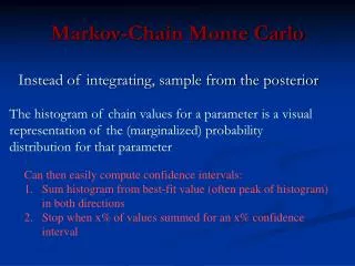
Markov Chain Monte Carlo. Gil McVean Tuesday 24 th February 2009. Bayesian inference. In Bayesian statistics we want to learn about the probability distribution of the parameters of interest given the data = the posterior

Markov Chain Monte Carlo
E N D
Presentation Transcript
Markov Chain Monte Carlo Gil McVean Tuesday 24th February 2009
Bayesian inference • In Bayesian statistics we want to learn about the probability distribution of the parameters of interest given the data = the posterior • In simple cases we can derive analytical expressions for the posterior • For example, if we have a beta prior: Beta(a,b) for a binomial parameter, after we have observed n successes and m failures, the posterior is also beta: Beta(a+n, b+m). The key here is conjugacy. Prior Likelihood Posterior Normalising constant
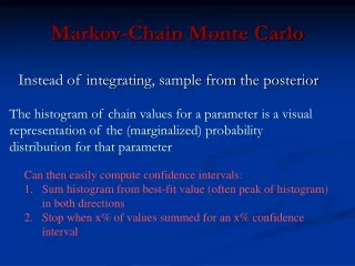
Monte Carlo methods • In many situations, the normalising constant cannot be calculated analytically • Typically this is true if we are dealing with multiple parameters, multidimensional parameters, complex model structures or complex likelihood functions • i.e. most situations in modern statistics • We can use Monte Carlo methods to sample from (and therefore estimate functions of) the posterior • Perhaps the most widely used method is called Markov Chain Monte Carlo, brought to prominence by a paper in 1990 by Gelfand and Smith.
Markov Chain Monte Carlo • The basic idea is to construct a Markov Chain whose stationary distribution is the required posterior • A Markov Chain is a stochastic process that generates random variables X1, X2, …, Xt, where the distribution i.e. the distribution of the next random variable depends only on the current random variable • Note that the Xi are typically highly correlated, so each sample is not an independent draw from the posterior • Thinning of the chain leads to effectively independent samples
Metropolis sampling • Gibbs-sampling is an example of MCMC that uses marginal conditional distributions. However, we do not always know what these are. • However, it is still possible to construct a Markov Chain that has the posterior as its stationary distribution (Metropolis et al. 1953) • In the current step, the value of the parameters is Xt. Propose a new set of parameters, Y in a symmetric manner; i.e. q(Y|X) = q(X|Y) • Calculate the prior and likelihood functions for the old and new parameter values. Set the parameter values in the next step of the chain, Xt+1 to Y with probability a, otherwise set to Xt
Some notation • I shall refer to the posterior distribution as the target distribution • The transition probabilities in the Markov chain I shall refer to as the proposal distribution; also known as the transition kernel • When talking about multiple parameters I shall refer to the joint posterior and the conditional distributions
An example • There are two types of bus: frequent (average arrival time = 5 mins) and rare (average arrival time = 10 mins). I see the following times • If I model the inter-arrival times as a mixture of two exponential distributions, I want to perform inference on the proportion of frequent and rare buses Number Arrival time
I will put a beta(1,1) = uniform(0,1) prior on the mixture proportion f • Starting with an initial guess of f = 0.2, I will propose changes uniform on f - e, f + e • (Note that if I propose a value < 0 or >1 I must reject it) • 50, 500 and 5000 samples from the chain give me the following results f f f iteration iteration iteration f f f
Under the bonnet • Consider a system in which a single parameter can take k possible values • My proposal is to select at random from one of the k-1 other possible values • Now suppose the system has reached its stationary distribution so that the probability of the chain being in a given state is proportional to its prior times its likelihood • Consider two states, i and j, with p(Xi) > p(Xj). The rates of flow in the two directions are Flow i to j Flow j to i
The small print! • If detailedbalance holds for every pair of states, the system remains in its stationary distribution • We just need to guarantee that the stationary distribution is reached • There are three requirements for Xt to converge to the stationary distribution • X must be irreducible. That is every state must be (eventually) reachable from every other state • X must be aperiodic. This stops the chain from oscillating between different states • X must be positive recurrent. This states that the expected waiting time to return to a state is finite and means that a chain will stay in its stationary distribution once it first reaches it
The Hastings ratio • A simple change to the acceptance formula allows the use of asymmetric proposal distributions and generalises the Metropolis result • Moves that multiply or divide parameters need to follow change-of-variables rules Sampling from an Exp(1) distribution Xt
Gibbs sampling as a special case • In Gibbs sampling we want to find the posterior for a set of parameters • Each parameter is updated in turn by sampling from the conditional distribution given the data and the current value of all other parameters • Consider the case of a single parameter updated using the Metropolis algorithm where the proposal density is the conditional distribution • In other words, the Gibbs sampler is an MCMC where every proposal is accepted • With multiple parameters you have to be careful about update order to ensure reversibility
Convergence • The Markov Chain is guaranteed to have the posterior as its stationary distribution (if well constructed) • BUT this does not tell you how long you have to run the chain in order to reach stationarity • The initial starting point may have a strong influence • The proposal distributions may lead to low acceptance rates • The likelihood surface may have local maxima that trap the chain • Multiple runs from different initial conditions and graphical checks can be used to assess convergence • The efficiency of a chain can be measured in terms of the variance of estimates obtained by running the chain for a short period of time
Watching your chain x = 0.1 Acceptance = 97% • Three chains, each sampling from an Exp(1) distribution with a uniform(-x, x) proposal distribution • Measure acceptance rates x = 1 Acceptance = 62% x = 10 Acceptance = 8%
The burn-in • Often you start a chain far away from the target distribution • Truth unknown • Check for convergence • The first few samples from the chain are poor representatives from the stationary distribution • These are usually thrown away as burn-in • There is no theory that says how much to throw away, but it’s better to err on the side of more than less
Other uses of MCMC • Looking at marginal effects • Suppose we have a multidimensional parameter, we may just want to know about the marginal posterior distribution of that parameter • Prediction • Given our posterior distribution on parameters, we can predict the distribution of future data by sampling parameters from the posterior and simulating data given those parameters • The posterior predictive distribution is a useful source of goodness-of-fit testing (if predicted data doesn’t look like the data you’ve collected, the model is poor)
Modifications • An important development has been to allow trans-dimensional moves (Green 1995), also known as Reversible Jump MCMC • Useful when looking for change points (e.g. in rate) along a sequence • Examples include looking for periods of elevated accident rate or genomic regions of elevated recombination rate • There are many subtle variants of basic MCMC that allow you to increase efficiency in complex situations (see Liu 2001 for many) Data Posterior probability of change in rate Time
A good read • Markov Chain Monte Carlo in Practice. 1996. eds. Gilks WR, Richardson S and Spiegelhalter DJ. Chapman & Hall/CRC. • Bayesian Data Analysis. 2004. Gelman A, Carlin JB, Stern HS and Rubin DB. Chapman & Hall/CRC. • Monte Carlo Strategies in Scientific Computing. 2001. Liu JS. Springer-Verlag. • Chris Holmes’ short course on Bayesian statistics • http://www.stats.ox.ac.uk/~cholmes/Courses/BDA/bda_mcmc.pdf