
Optimal Groundwater Remediation
E N D
Presentation Transcript
Optimal Groundwater Remediation Laura Place Taren Blue
Outline • Background • What is Groundwater Remediation • Major Contaminants and Contamination Areas • The Remediation Process • Treatment Methods • Mathematical Models • Optimization • Completed Work • Fluid Flow Modeling • Plans and Recommendations for Future Work
Background • Groundwater Remediation • Removal of contaminants from a water supply • Standards set by the EPA • Several methods for treatment • Existing • Experimental • Optimization • Mathematical models
Background • Sources of contamination • Industrial & agricultural • Storage tanks • Septic systems • Landfills • Hazardous waste sites • Road salts • Refinery operations • Mining • Other chemicals
Where are the Problem Areas? Nitrates Arsenic Hard Water VOCs
Optimization • Goals • Minimize the remaining contaminants • Minimize cost • Costs minimized are unique to the model • Other goals are also unique to the specific model • Optimizing the pump treat inject method (PTI) • Number of wells • Well configuration
What are the Choices? • “Dilution is not the solution!!!” • Inexpensive but never resolves the problem • Pump, Treat, Inject method (PTI) • Pump contaminated water from the source (the plume) • Treat the water • Inject treated water back into the aquifer
Treatments • Existing treatment methods • Ion exchange chromatography • Membranes • “Point of service” treatment • Bioreactors • Adsorption • In situ bioremediation • Liquid-liquid extraction • Surfactants
Challenges of Remediation • Plume • Unknown flow patterns • Unknown concentration profiles • Nonuniformities in concentration • Unknown position • Uncertainty in composition • Unknown size • Geological uncertainty
Problems and Affect on Treatment ***Modeling of the aquifer depends on many of these parameters. Therefore, all of these issues also become a problem in mathematical modeling.
PTI • Has many parameters • Number and location of wells • Few large wells • Many small wells • Pumping Rate • Concentration of contaminants in treated water • Can vary well arrangement with time • For optimization – Need a model!
Well Position and Treatment Four different well arrangements. ***Concentration profile of the plume is affected by location of pumping and injection wells.
Steps Completed in Optimization • Analytical Model • Euler Approximation • Optimization for minimum cost • Initial Fluid Flow Modeling and Analysis • Refined Fluid Flow Modeling and Analysis • Optimization for minimum contamination
Set Up Euler Approximation • Where • dc/dt is the change in concentration with time • Fp is the pumping rate • cin is the concentration into the slice • cout is the concentration out of the slice • Vslice is the volume of the slice
Euler Method Model • Calculates total remediation time • Uses inputs for: • Volume of the plume • Time steps • Flow rate • Initial concentration • Desired end concentration • Calculation in each cell loops until the change in outlet concentration is < 0.0001
Euler Results t1 t2
Fluid Flow Analysis Arrangement Example of one arrangement – multiple outlets with one inlet
Fluent • Calculate mass flow rates in the plume • More accurate approximations of concentration profiles • Characterize fluid flow in the aquifer • Vary well arrangement • Vary number of injection and extraction sites • Vary pumping rate
Geometry - Gambit • 1st “draw” geometry in Gambit • Create injection and extraction locations which may be turned on or off. • For off – face is treated as a wall • For on – face is designated either mass inlet or outflow • Each face is labeled by location
Generic Geometry 10 20 10 A B C D E F G 1 2 3 4 5 6 7
Define Geometry in Fluent One outlet One inlet
Imaginary Planes A B C • Fluent analyzes flow patterns through planes I J K D L M N E O P Q F G H
Example of Fluid Flow Field in Fluent Flow rate of 50 kg/s
Example of Fluid Flow Field in Fluent Flow rate of 5 kg/s
Example of Velocity Contours Flow rate of 5 kg/s
Excel • Results from Fluent imported into Excel
Mass Balance C-18 C-14 C-10 Negative flux or positive flux dictates which concentration to use in the mass balance
Remediation Time and Flow Rate (2,1) (1,1) (4,1) (1,4) (4,4) (2,2) (1,2)
Conclusions of this Model • Imaginary planes give an accurate estimate of flow through the aquifer • Flux through the planes can be used to describe concentration profiles with time • This model allows for understanding of general flow patterns with configuration • Gives basis of comparison for future modeling techniques
New Modeling Strategy • Pipes in the top of the aquifer • More realistic injection modeling • Flow characteristics re-evaluated • Several plume types evaluated • Non-uniform initial concentrations • Different shapes • Injection and extraction varied with time • More realistic aquifer shape
Naming the Wells 1 2 3 4 5 6 7 A B C D
Planes Through the x-direction -18 -14 -10 … 18
Horizontal Planes Horizontal planes also named individually for x, y and z location in the aquifer.
Model Aquifer with Non-Uniform Concentration • 3 plumes analyzed
Schemes for TreatmentPlume 1 Step 1 Step 2 Step 3
Schemes for TreatmentPlume 2 Step 1 Step 2 Step 3
Schemes for TreatmentPlume 3 Step 1 Step 2 Step 3