Overview of Orbit Measurement and Correction Techniques in HERA and Related Colliders
380 likes | 513 Vues
This document provides a comprehensive overview of orbit measurement and correction techniques utilized in high-energy particle colliders, notably HERA and other systems. It covers topics such as 1:1 steering, beam-based alignment (BBA), dispersion-free steering, and orbit feedback mechanisms. The text elaborates on the impact of relative alignment errors on beam performance, detailing multipole field expansions and their implications on beam dynamics. The effect of quadrupole and sextupole misalignments and solutions for optimizing beam trajectories through calibration and steering feedback methods are also discussed.

Overview of Orbit Measurement and Correction Techniques in HERA and Related Colliders
E N D
Presentation Transcript
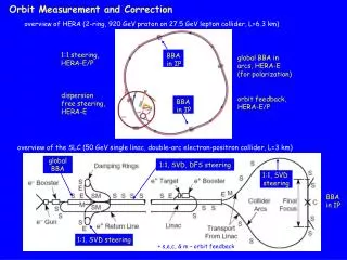
Orbit Measurement and Correction overview of HERA (2-ring, 920 GeV proton on 27.5 GeV lepton collider, L=6.3 km) 1:1 steering, HERA-E/P BBA in IP global BBA in arcs, HERA-E (for polarization) dispersion free steering, HERA-E orbit feedback, HERA-E/P BBA in IP overview of the SLC (50 GeV single linac, double-arc electron-positron collider, L=3 km) global BBA 1:1, SVD, DFS steering 1:1, SVD steering BBA in IP 1:1, SVD steering + s,e,c, & m – orbit feedback
overview of RHIC (2-ring, 250 * 250 GeV proton-proton collider; 100 GeV ion-ion collider, L=6.8 km) 1:1 and SVD steering BBA in IP BBA in IP
Introduction types of relative alignment errors and their effect on the beam: z multipole field expansion x bn 0, an= 0: bn=0, an 0: “skew” (e.g. rotated by 45° component) “normal” (e.g. up- right) component p. 65 ,below Eq. 2.106 Lorentz force example: (normal) quadrupole n=1: Bz+iBx=(b1+ia1)(x+iz) Bz=b1x Bx=b1z Fx = -qvBz = -qvb1x Fz = qvBx = qvb1z B F for x0, the field experienced is that of a dipole the off-axis beam sees the next-lower order field (“feeddown effect”)
Bz/b0 normal dipole Bz=b0 Re(x+iz)0=b0 Bx=b0 Im(x+iz)0=0 x Bz=a0 Im(x+iz)0=0 Bx=a0 Re(x+iz)0=a0 “skew” dipole Bz/b1 Bz=b1 Re(x+iz)=b1x Bx=b1 Im(x+iz)=b1z normal quad x Bz=a1 Im(x+iz)=a1z Bx=a1 Re(x+iz)=a1x “skew” quad Bz/b2 Bz=b2 (x2-z2) Bx=2b2xz normal sextupole (z=0) skew sextupole Bz=2a2xz Bx=a2(x2-z2) x x = xco + xβ + x dispersive orbit defined by magnetic focussing closed orbit off-axis beam sees sextupole, quadrupole, and dipole fields example: z=0, x=0: Bz/b2=(xco2+2xxco+x2xco2)
In addition to perturbing the design optics, off-axis in quadrupole dipole field: generates dispersion D~1/ρ leads to dispersive emittance growth when ≠ 0 since x =η and x ~ <x2>1/2 (here x=transverse position offset) causes sampling of nonlinear fields, contributes to emittance growth leads to beam depolarization when magnetic moment of particle μ experiences a transverse deflecting field B off-axis in sextupole quadrupole and dipole fields: introduces additionally β-beats (gradient errors), vertical dispersion, betatron coupling, … off-axis in accelerating structures wakefield kicks: dilution of projected beam emittance since different particles within the bunch follow different trajectories solutions: alignment (by surveying) beam-based alignment steering feedback focus of this lecture
famous question: “where is zero?” beam centroid position with respect to the reference axis xco = xd + xb + xm quadrupole misalignment measured beam position BPM electronic and/or misalignment offset the “answer” depends on application chosen: orbit correction method consequence(s) BBA of single elements and global BBA one-to-one steering SVD steering dispersion-free steering absolute position of beam wrt magnet center - best solution (but invasive, time consuming, and for global BBA, complicated) BPM values zeroed, corrector values (and ) nonzero - beam may be still off-axis BPM readings and corrector values minimized using empirical weighting of the unknown offsets BPM reading and corrector values minimized with additional constraints given by dispersive orbits
Beam-based alignment of single elements: quadrupoles typical residual alignment errors after surveying: ~ (100-200) μm typical quadrupole alignment tolerances in storage rings (i.e. synchrotron light sources): ~ 10 μm circular collider IPs (i.e. B-factories, HERA, LHC) ~ 5 μm linear collider IPs (i.e. NLC, TESLA) < 1 μm Beam-based alignment determines the relative offset between magnet centers and nearby BPMs. If the offsets are sufficiently stable, then simple orbit cor- rection (steering) can be used to maintain a well-centered orbit. BBA using quadrupole excitation (xb and xq are unknown) dipole kick xb≠0 xb=0 xb=0 s s s xq≠0 xq=0 xq=0 nominal case (after steering “flat”) ideal case (with misalignments) ideal case
single-pass measurement (transport line or linac): dipole kick (for horizontally focussing quadrupole) Θ=K·xq (in 1/m) change in integrated field B(I), where B(I) depends on magnet properties quadrupole misalignment ρ(eVs/m) m Vs/m3 example from the TESLA test facility (courtesy P. Castro, 2000) total quad current variation of ~ 5% triplet quad center corrector s x (mm) slope ~ R12 since x~ (Icor) BPM (set field to zero) independent of absolute BPM position (and electronic offsets) K minimum displacement please replace quad with cor in figure caption 3.6, p. 74 Icor (A)
multiple-pass measurement (circular accelerator): warning: new analyses… s Θ≈K·xq- K x + O (K· x) xq BPM #1 BPM #2 (as before) change in the closed orbit offset at the quadrupole solve iteratively using expression for the c.o.d. at the location of the kick (Eq. 2.34): solving for x: and inserting back into first eq. above: example from SPEAR (courtesy J. Corbett, 1998) BPM #1 quad center x=difference orbit measured at BPM BPM #2 quadrupole shunt circuitry (allowing variation of single quad given multiple magnets per power supply) xq=orbit offset at quadrupole (varied using local bump)
quadrupole gradient modulation (LEP) modulation of single quadrupoles with (non-resonant) discrete frequencies example from LEP(courtesy I. Reichel, 1998) response of beam to modulation of four different quadrupoles natural orbit drift and correction at a single quad (time scale, 6 hrs) orbit correction ~ 1 μm FS orbit variation measured at BPM close to modula- ted quad using position jitter (time scale short) relative offset FFT of turn-by-turn BPM measurements minimum gives relative BPM offset (~200 μm)
Beam-based alignment of single elements: sextupoles recall (normal sextupole): Θx~Bz=b2 (x2-z2) Θz~Bx=2b2xz Possible approaches (using sampled quadrupole field): 1. use additional quadrupole trim windings, mounted on the sextupoles, quadrupole-based BBA (KEK) – (assumes coinciding magnetic centers of trim windings and sextupole) 2. measure shift in betatron tune vs sextupole strength (PEP-II, HERA,…): θx~ ( xβ+ xco )2 - ( zβ+ zco )2 ~ … + xβxco + … zβzco + … need for each sextu- pole an indi- vidual power supply off-axis in x (xco≠0) θx~xβ (quadrupole field); similarly in z 3. measure tune separation near the difference resonance vs sextupole strength (NLC): θz ~ … + xβzco + … off-axis in z (zco≠0) θz~xβ (skew quadrupole field)
Possible approaches (using sampled dipole field): 1. using local orbit bumps (KEK,DESY): horizontal sextupole alignment: θx = -0.5 Ks (xbump-xs)2 θz = -0.5 Ks (xbump-xs)zs vertical sextupole alignment: θz = Ks (x0-xs)(zbump-zs) xs and zs are the sextupole offsets change strength of all sextupoles by Ks measure induced orbit change repeat for different bump amplitudes independent of the number of sextupoles driven by a single power supply x0 is a preferably large horizontal orbit offset (for enhanced sensitivity) 2. using induced orbit kick vs sextupole position (KEK B-factory, SLAC FFTB) example from the FFTB (courtesy P. Tenenbaum, 1998) sextupoles mounted on precision movers, measure quadratic change in closed orbit (transfer line or linac) center at dxb/dxm=0
Beam-based alignment of accelerating structures s x couple out power at natural resonant frequencies of the structure (higher-order modes) if x,y≠0 using output coupler example from the ASSET experiment at SLAC (courtesy M. Seidel and C. Adolphsen, 1998) signal amplitude at fc = 16 GHz ~ 7.5 MHz (after mixing) T (structure central axis to beam position infered from BPMs) 90 relative position offsett phase (deg) please fix scale on bottom plot of Fig. 3.10, p. 79 -90
Lattice diagnostics and R-matrix reconstruction simple FODO lattice quadrupole with BPM corrector dipole point-to-point transfer matrix: measure R12=dx/dx’ plot x=R11x+R12x’max method I “jitter data” plus careful 2-dimensional error propagation, parasitic method II 2-point fit x(x’=0), x(x’≠0) or, for better measurement (smaller error), x vs x’
example: linac-to-ring transfer line (SLC) angular deflection (“kick”) due to dipole: since then Bρ=magnetic rigidity =E(GeV)/0.3 [T-m] =p (MeV)/300 [T-m] slope: measurement at a single location as the strength of an upstream corrector is varied to probe all elements in the beamline, need a second corrector dipole separated in betatron phase by π/2
example: linac-to-ring transfer line (SLC), continued: “fitted” R12 concept: acquire data using all available BPMs while one upstream corrector is varied then minimize calc fitting for the best incoming orbit given by x1, x1’ data (solid line): measured trajectory fitted (dashed line): x1 + R1jxj’ (using R1j measurements and x1 fitted) y(s) x(s) 60 m, 20 BPMs 60 m, 20 BPMs Comparison allows for localization of optics errors and BPM errors (these BPMs may then be excluded in subsequent steering procedures)
Suppose there is poor agreement between expectation and measurement. Possible causes include: optical errors (including knowledge of B-fields) incomplete model corrector and BPM gain/polarity (and location) errors example:lattice diagnostics in the main SLC linac (courtesy T. Himel and K. Thompson, 1999) expanded R-matrix: energy dependence of the point-to-point transfer matrix obtained using a Taylor series expansion to first order in the energy with Nk(=240)=total number of klystrons, Ek=energy gain per klystron with Nk(=30)=total number of sectors, Ek=energy gain per sector data (solid line): measured trajectory fitted (dashed line) as before with linear scaling of beam energy evidence of 180° phase shift in center of linac 1500 m, 300 BPMs
Possible causes for discrepancy chromatic phase advance in a FODO cell: with (90° FODO cell) if not taken into account, expect a 90° cumulative error with =2.5%, =30sectors●2π/sector unknown energy errors procedure used for further analysis: 1. measure xm(s) versus the applied deflection 2. select a set of Ek’s 3. compute computed measured 4. iterate for minimum 2
result model still lacks all physics input (i.e. energy spread variation along the linac not taken into account) the model offers reduced complexity (30 fit parameters, which are well con- strained given the ~1200 R-matrix elements) the estimated energy error ~30%, greatly exceeding the estimated uncertainty before the energy fit data (solid line) fitted (dashed line) (bad BPMs) after the energy fit data (solid line) fitted (dashed line) Nevertheless, the predictive power of the model is very useful; e.g. for localization of BPM and klystron phase errors
Beam Steering Algorithms review:so far we have discussed beam-based alignment of single elements which, while accurate, is time consuming and so used most often during early stages of accelerator commissioning and in interaction regions, where single-element alignment tolerances are most critical lattice diagnostics which is often needed prior to being able to implement automated steering algorithms which may be model-dependent and are significantly less prone to errors if “bad BPMs” are excluded from the data samples until now (in the discussion of BBA and lattice diagnostics) only the coherent motion of the bunch centroid (center of charge) has been considered Beam steering is applied over long regions of the accelerator and is significantly more time-efficient than BBA of single elements. Note that while the center of charge is measured by the BPMs, the best beam steering algorithms ideally minimize the projected beam emittance. Again (with x = horizontal or vertical), x = xco + xβ + x dispersive orbit orbit defined by magnetic focussing closed orbit The emittance εx ~ σx2/β, where σx = <x2>1/2 = <(xco+ xβ + x)2>1/2 which contains for example a dispersive term σ=<x2>1/2=2<2>1/2
“One-to-One” steering (linear least-squares algorithm) Beam is steered to zero the transverse displacements measured by the BPMs. The BPMs are typically mounted inside the quadrupoles (where the β-functions are largest). closed bump that would minimize the BPM readings (but would also generate dispersion) indices i denote each corrector kick Beam position measured at a downstream BPM (denoted by subscript, j): ( Fi-Fj ) m is the total number of BPM measurements In matrix form with ( ( n is the total number correctors Solving the matrix equation: x is the vector containing the BPM measurements or Θ is the vector containing the unknown kick angles
Again , the solution is given by Here, θ is an (n1) matrix [n=number of correctors] M is an (nm) matrix x is an (m1) matrix [m=number of BPM readings (per plane of interest)] If m>n, the matrix M is overdetermined m=n, the matrix M is square and the solution is simply θ=M-1x m<n, the matrix M is underdetermined and more measurements are needed (to ensure that the number of unknowns is at least equal to the number of measurements). To constrain the solution in this case, some parameter (e.g. the beam energy) needs to be varied and the measurement repeated (however, the measurement fails to be noninvasive)
minimization procedure: The solution to the matrix equation can equivalently be found by minimizing fitting function with unknowns Θi (i = number of unknown kicks) measurements (j = number of BPM measurements) i.e. vary (possibly numerically) the unknowns θi given the BPM measurements xj and the assumed transfer elements Mji so that the relation holds (as closely as possible) i.e. (algebra) (reorganizing terms) This equation, expressed in matrix form, is equivalent to the result from before:
Global beam-based steering Take into account now that the electrical center of the BPMs ≠ center of quadrupole xm xbpm xq beam position wrt quad center sum over all upstream quadrupoles beam position wrt reference axis beam position wrt reference axis transported between quad (j) and quad (j+1) beam position wrt quad center transported between quads (j) and (j+1) = beam position at quad k
again rearrange terms sum over upstream quadrupoles function to be minimized: measurements fitting function with unknowns xq, xbpm, and (x0,x0’) Since the number of measurements is about ½ the number of unknowns, an independent set of measurements is required. One possibility is to scale the lattice (all quadrupole and corrector strengths) and repeat the measurement.
Singular valued decomposition (SVD) Global orbit correction using the SVD algorithm offers the advantage of reducing not only the rms of the BPM measurements, but also the rms of the applied corrector strengths. Correctors compensating (or “fighting”) one another generate unwanted dispersion. This powerful algorithm may also be used in application to orbit feedback, dispersion-free steering, and in the computation of multiknobs. [caveat: “reversibility” in practical applications] matrix of corrector kick angles, (n1) matrix Matrix equation to be solved: measured orbit displacements, (linear) orbit response matrix, (m1) matrix (mn) matrix m=number of BPM readings n=number of correctors If m>n, the matrix A may be decomposed (easily using matlab, for example) U is an(mn) matrix V is an(nn) matrix The column vectors of U and V are orthonormal satisfying (In is the (nn) identity matrix)
Again, A is an (mn) matrix m=number of BPM readings n=number of correctors m=n: A is square matrix and the solution for the correctors is If none of the wi are zero, the solution is unique (example to follow). If one or more of the wi are zero (degenerate case), there may not be an exact solution. In this case, replace 1/wi by zero which gives still the solution in the least squares sense; i.e |A●θ-x| and |θ|2 are minimized. m<n: Add rows with zeroes to the vectors and matrices in x=Aθ until the A matrix is square and apply the SVD algorithm as just described (again a degenerate case) m>n: SVD solution will agree with the result of the least-square fit
Numerical example of the SVD algorithm x c1 - c2 =π correctors s 1 - c2 =π/2 BPMs 1 - 2 = π using x=R12θ and plus a convenient normalization Matrix equation to be solved which may be decomposed as with solution Θ=A-1 x Given the above geometry, there is no exact solution for placing the beam at arbitrary desired positions at both BPMs. However, there is an SVD-solution. Suppose we want to steer the beam to xt1=1 and xt2=0. Then The positions at the BPMs with this solution are x1=1/2 and x2=-1/2. With this solution, the quadratic distance to the target values ∑i(xti-xi)2 and the corrector strengths ∑jθj2 are minimized.
Dispersion-free steering (Raubenheimer, Ruth) one-to-one steering – a first step in orbit correction but imperfect since dispersive errors may be generated global beam-based alignment of quadrupoles – works well at low beam currents where there is no wakefield-generated dispersion wakefield bumps – more local but highly sensitive to small perturbations dispersion-free steering – even more local correction of dispersive errors including dispersive errors arising from transverse wakefields absolute orbitt: again, i=1,2,…,n, n = no. correctors j=1,2…,m m = no. BPMS including now the energy-dependence (adiabatic damping) To constrain the system (taking into account the additional unknown energies), the beam energy may be changed (not so easy) or the lattice (quadrupoles and correctors) may be scaled to mimic a change in beam energy. Then difference orbit: K is the quadrupole strength factor missing in text, Eq. 3.41 tmeasured center-of-charge. please replace “for a deflection applied in” with “between” before Eq. 3.41, p. 92
Again, absolute orbit difference orbits minimize the absolute orbit and the difference orbit simultaneously: (N1) (2MN) (2M1) SLC experience: initially, solution overconstrained by scaling lattice in steps (K/K=0%, -10%,-20%, -30%, +5%, 0%); later, the problem of hysteresis was overcome (Raimondi) by measuring the orbits of the e+ and e- beams (which is equivalent to K/K=200%)
simulated orbit and dispersive emittance with single 100 μm quadrupole offset (courtesy R. Assmann, 2000) ~ 200σβ simulated orbit and dispersive emittance with single 100 μm structure offset (courtesy R. Assmann, 2000) ~ (3-4)σβ (single particle model)
simulated orbit and dispersive emittance with quadrupole and structure offsets after application of one-to-one steering (courtesy R. Assmann, 2000) solid line: quadrupole offset dashed line: structure offset ~ (3-4)σβ
measured dispersive orbits before correction =1.0 =0.9 • Remarks: • after DFS, the maximum • orbit difference (neglecting • the bad BPM) was reduced • from ~ 1.5 mm to < 200μm • 2) after DFS, the rms of the • absolute orbit was larger – • suggesting that significant • BPM and/or quadrupole • misalignments were still • present =0.7 =0.8 after (3 intera- tions) of DFS steering
measured absolute orbits after two-beam dispersion free steering
errors typical error sources and their rms contributions: σ(xj)BPM resolution <10 μm σBPM BPM misalignments ~100 μm σsys systematic errors (jitter and drift) ~20 μm sum over j BPM measurements to propagate errors, introduce a weighting function m denotes the different error sources function to be minimized: one-to-one steering beam-based alignment dispersion-free steering (recall x is a vector with positions and orbit differences, the Mij are transfer matrix elements with and with- out the energy-equivalent scaling)
Error evaluation with dispersion-free steering (Assmann) function to be minimized: goodness-of-fit parameter defined with emphasis on the leading error sources: BPM misalignments cancel in the measure- ments of the difference orbits systematic errors contribute less than the alignment errors in measurements of the absolute orbits rms of vertical beam positions: in absence of “deterministic fits” (number of unknowns = number of measurements with no degener- acies), skill and experience are required in determining optimum weighting factors: weighting by disper- sion cor- rection weighting by orbit correction
Summary: Using the multipole field expansion, we discussed relative alignment errors and (some of) their effects on the beam (e.g. “feed-down effect”) Typical magnet-to-beam alignment tolerances, storage rings (i.e. synchrotron light sources): ~ 10 μm circular collider IPs (i.e. B-factories, HERA, LHC) ~ 5 μm linear collider IPs (i.e. NLC, TESLA) < 1 μm are considerably tighter than what can be achieved by precision alignment (surveying) which is on the order of (100-200) m To overcome these difficulties, beam-based alignment and beam steering are used We reviewed various methods of beam-based alignment of single magnetic elements including various methods for aligning quadrupoles and sextupoles. As a precursor to beam steering methods, “lattice diagnostics” was presented, which is yet another method for localizing optics and BPM errors (the “bad BPMs” would then be excluded from steering algorithms) An example was presented, whereby an incomplete model with known shortcomings (as aften the case) could nonetheless provided information on optical and BPM errors
The steering method of choice (incidentally: unavoidable in large accelerators) depends on many factors including availability and reliability of BPMs relative importance of well-controlled orbits versus investment of effort relative importance versus investment of beam time prevailing conditions (i.e. presence of wakefields at high beam currents) Common methods of beam steering were described and algorithms were given for numerical analysis The methods presented included: one-to-one steering global beam-based alignment SVD steering dispersion free steering Aspects of the mathematics were illustrated using simple examples 2-corrector / 2-BPM 2 minimization and SVD solution Completely overdetermined systems (as nowadays typical) require additional constraints (represented by the “weighting factors”, which implies non-deterministic solutions which require experience and skill to optimize Once optimal orbits have been determined, orbit feedback (not yet presented) may be used to maintain the orbits (provided that they don’t drift with time) Tutorial on SVD and Least-Squares including “bad BPMs” and RHIC data available on request