Coherent X-ray Imaging (WBS 1.3) Sébastien Boutet

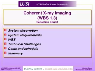
1. Coherent X-ray Imaging(WBS 1.3)Sébastien Boutet • System description • System Requirements • WBS • Technical Challenges • Costs and schedule • Summary

2. Science Team • Specifications and instrument concept developed with the science team. The CXI team leaders • Janos Hajdu, Photon Science-SLAC, Uppsala University (leader) • Henry Chapman, LLNL • John Miao, UCLA

3. Molecular Structure Determination by Protein Crystallography • Molecular structure is crucial for medical applications. • Inability to produce large high quality crystals is the main bottleneck. • Radiation damage is overcome by spreading it over 1010 or more copies of the same molecule.

4. Coherent Diffractive Imaging of Biomolecules One pulse, one measurement Particle injection XFEL pulse Noisy diffraction pattern Combine 105-107 measurements into 3D dataset Gösta Huldt, Abraham Szöke, Janos Hajdu (J.Struct Biol, 2003 02-ERD-047)

5. Conceptual Design of CXI Instrument Particle injection Pixel detector Intelligent beam-stop (wavefront sensor) LCLS beam (focused, possibly optically compressed) Optical and x-ray diagnostics To Time Of Flight (TOF) mass spectrometer Readout and reconstruction

6. Short pulses Instantaneous snapshots with no thermal fluctuations. Limited radiation damage during the exposure. High brightness Good signal-to-noise with a single shot. Smaller samples. Spatial coherence Elimination of incoherent scattering which contributes to sample damage but not to the signal. Scientific programs X-ray-matter interactions on the fs time scale. Validation of damage models. Structure determination from nanocrystals of proteins. Imaging of hydrated cells beyond the damage limit in 2D. Imaging of nanoparticles. Structure determination of large reproducible biomolecules. Structure determination of reproducible protein complexes and molecular machines. CXI Science at LCLS

7. CXI SCOPE - WBS 1.3

8. System Specifications Photon Shutter Primary Slits Compressor Attenuators Focusing Lenses Pulse Picker Diagnostics FEH Hutch 5 Secondary Slits KB Mirrors Secondary Slits Diagnostics Sample Environment Particle Injector Electron-Ion TOF Detector Stage Wavefront Sensor Beam Dump

9. Coherent X-ray Imaging Instrument Coherent X-ray Imaging Instrument Particle injector Electron/Ion TOF Cryo-goniometer 10 micron Be lens (not shown) Wavefront sensor X-ray Pulse compressor (not shown) 1 micron KB system 0.1 micron KB system Sample Chamber with raster stage LCLS detector

10. CXI System Description • 1.3.1 Physics support and engineering integration • 1.3.2 X-ray optics • 1.3.3 Sample environment • 1.3.4 Laboratory facilities • 1.3.5 Vacuum system • 1.3.6 Particle injector • 1.3.7 Installation

11. 1.3.2 X-ray Optics Focusing optics Pixel detector Beam-stop Sample handler KB Mirrors 1 µm 0.1 µm Be Lens Monochromator/ pulse-compressor Offset mirror pair FEL source Sample chamber & diagnostics f1 µm f0.1 µm zd zs ≈ 400 m Image reconstruction

12. 1.3.2 X-ray Optics • 1.3.2.2 Mirror system (1 µm and 0.1µm KB) • KB mirrors have produced 50 nm focuses of SR(Yamauchi et al., SRI 2006). • Can use bent plane mirrors – plane mirrors most accurate polishing. • Achromatic focusing. • Use B4C as coating • Damage resistant • Good reflectivity

13. 1.3.2 X-ray Optics • KB Pair for 1 μm focus • Grazing angle 0.2 Deg • B4C coating • Horz. Mirror 20 cm • Vert. Mirror 10 cm • Focal spot size (FWHM in microns) • Horz: 0.6 • Vert: 0.9

14. 1.3.2 X-ray Optics • KB Pair for 0.1 μm focus • Grazing angle 0.2 Deg • B4C coating • Horz. Mirror 20 cm • Vert. Mirror 10 cm • Focal spot size (FWHM in microns) • Horz: 0.097 • Vert: 0.083

15. 1.3.2 X-ray Optics • 1.3.2.1.2 – Pulse picker • Permit LCLS operation at 120 hz • Single pulses for samples supported on substrates • Reduced rate. Example :10 hz operation • High damage threshold • Use rotating discs, concept already in use at ESRF • Combined with a ~0.1 sec shutter. • Commercially available millisecond shutter. • Allows any pattern of pulses. • Life duty cycle limitations

16. 1.3.2 X-ray Optics Focusing optics Pixel detector Beam-stop Sample handler KB Mirrors 1 µm 0.1 µm Be Lens Monochromator/ pulse-compressor Offset mirror pair FEL source Sample chamber & diagnostics fBe lens zd zs ≈ 400 m Image reconstruction

17. 1.3.2 X-ray Optics • 1.3.2.2 Beryllium lens focusing optic • ~ 10µm FWHM focal spot size • Positioning resolution and repeatability to 1 µm

18. 1.3.2 X-ray Optics • 1.3.2.3 Precision Slit System • Positional resolution and repeatability – 1 µm • High damage threshold Boron Carbide Slit Blade Tungsten Alloy

19. 1.3.2 X-ray Optics • Apodized edge slits • Soft edges to minimize slit scatter. • Used as cleanup slits just before the sample • Remove the halo around the focus • Positional resolution and repeatability : 1 µm • Made of etched Si wedges

20. 1.3.2 X-ray Optics • 1.3.2.4 - Attenuators • Variable, up to 106 reduction • High damage threshold : Be or B4C • Highly polished to minimize distortions of the wavefront

21. 1.3.2 X-ray Optics • 1.3.2.5 Pulse Compressor • x10 reduction in pulse length • Provide optics, precision motions • Use when LCLS produces chirped pulses

22. 1.3.2 X-ray Optics 476 µm Henry Chapman LLNL

23. 1.3.2 Level 4 Direct Costs

24. 1.3.3 Sample environment • 1.3.3.1 Sample chamber • Vacuum better than 10-7 torr • Sample raster stage • Aperture raster stage • Cryo-goniometer • Optical diagnostics

25. 1.3.3 Sample environment • 1.3.3.1 Sample Chamber (cont.) • Vacuum • Assumptions: • ‘Unshielded’ beam path of 10 cm for 1 µm2 beam • Biomolecule ~ 500kDa ~ 5 x 104 atoms • Background scatter 1% 500 atoms in path • Atoms in background gas same z as in the molecule p ≤ 1 x10-7 torr

26. 1.3.3 Sample Environment • 1.3.3.1 Sample Chamber (cont.) • Sample raster stage • Aperture raster stage • Cryo-goniometer • Adapted from cryo-EM • All motion drives outside vacuum • In use on SR sources for STXM • Provides full angular-spatial degrees of freedom to collect 3D data

27. System Specifications

28. 1.3.3 Sample environment • 1.3.3.2 Ion TOF • 1.3.3.3 Electron TOF • 3 x1012 photons in 100 nm spot • (a) 2 fs pulse • (b) 10 fs pulse • (c) 50 fs pulse • Provide diagnostics to understand the ‘explosion’ • Electron and Ion ToF detectors • able to resolve single atom fragments (1 AMU) • 1/1000 in electron energy

29. System Specifications

30. Real space samples:x Smallest period sampled: 2x = d or fmax = 1/d Oversampling (per dimension):s Array size:N = D s / x = 2 D s / d 1.3.3.4 Precision Instrument Stand The number of pixels fixes the resolution for a given particle size and oversampling ratio N x fmax f x D = N x / s 1.3.3 Sample Environment

31. 110 m pixels 2 = 30º zd zd =1450 mm, 760 pixels D = 1000 nm d=5.2 nm zd = 83.6 mm, 760 pixels D = 57 nm d=0.3 nm 1.3.3 Sample Environment • 1.3.3.4 Precision Instrument Stand (cont.) • Detector size and distance fixes resolution.

32. 1.3.3 Sample Environment • Tiled detector, permits variable ‘hole’ size: • Ideally the hole is ~ x2 bigger than incident beam at most • Dead area at edges of detector tiles limits minimum ‘hole’ size • Alternate approach: larger ‘hole’ and a single tile for forward direction • Simulations required ‘Hole’ in detector to pass Incident beam

33. Detector Options • Fixed hole size • Limits resolution achievable for large objects • Individually moveable modules to get higher resolution farther from sample • Fill in missing data with wavefront sensor data

34. 1.3.3 Level 4 Direct Costs

35. 1.3.4 Hutch Utilities & 1.3.5 Vacuum • 1.3.4 Laboratory Facilities • 1.3.4.1 Electrical • LCLS provides utilities to hutch • Distributing utilities within hutch - LUSI • 1.3.4.2 Control Room Furniture • 1.3.4.3 Hutch Furniture • 1.3.4.4 Radiation Physics • 1.3.5 Vacuum system • 1.3.5.1 Hardware - flanges, pumps • 1.3.5.2 Bellows • 1.3.5.3 Spools • 1.3.5.4 Supports for all systems

36. System Specifications

37. 1.3.6 Particle Injector • Aerodynamic lens: stack of concentric orifices with decreasing openings. • Can be used to introduce particles from atmosphere pressure into vacuum • Near 100% transmission • Creates a tightly focused particle beam. Final focus can be as small as ~10 mm diameter

38. 1.3.7 Installation • 1.3.7 Installation • 1.3.7.1 Non-recurring engineering • 1.3.7.2 Installation LCLS CD-4a • 1.3.7.3 Installation LCLS CD-4b • 1.3.7.4 Complete Installation LUSI CD-4a

39. Hartmann Wavefront Sensor Hartmann Plate 2D Detector Focusing Optic Focal Plane W FEL Beam w0 f D L * Requires a defocusing optic

40. Diffractive Wavefront Reconstruction • The oversampled diffraction pattern of the focus is measured. • The focal spot is iteratively reconstructed by propagating the wave from the optic to the focus and then to the detector plane. • The constraints are applied at the optic and detector planes. Attenuator 2D Detector Focal Plane Focusing Optic W FEL Beam w0 f L

41. Other X-ray Diagnostics (WBS 1.5) • Multiple pop-in diodes to check alignment of different optics • Non destructive Be foil backscattering can monitor intensity during measurement. • Place upstream of sample • Possible distortions of wavefront Pop-in diode Thin Be backscattering beam monitor

42. Risks

43. CXI Schedule in Primavera 3.1

44. CXI Milestones CD-1 Aug 01, 07 Conceptual Design Complete Oct 03, 07 CD-2a Dec 03, 07 CD-3a July 21, 08 Phase I Final Design Complete Aug 12, 08 Receive Sample Chamber Nov 11, 08 Receive Focusing Lenses Feb 26, 09 Receive Pulse Picker Mar 13, 09 Phase I Installation Complete Aug 26, 09 CD-4a Feb 08, 10

45. Cost Estimate

46. 1.3 Level 3 Costs (M$)

47. WBS 1.3 - CXI • Cost estimate at level 3 by fiscal year –

48. Summary • Instrument concept advanced • 100% of Letters of Intent are represented in instrument concept • Instrument concept is based on proven developments made at FLASH and SR sources • Initial specifications well developed • Ready to proceed with baseline cost and schedule development