Download
1 / 63
630 likes | 646 Vues
This course explores the principles and tools of computational photography, including image formation, camera parameters, image processing techniques, and future directions in smart cameras. Topics include gradient domain operations, graph cuts, image reconstruction, and more.

E N D
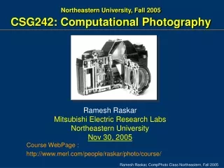
Northeastern University, Fall 2005CSG242: Computational Photography Ramesh Raskar Mitsubishi Electric Research Labs Northeastern University Nov 30, 2005 Course WebPage : http://www.merl.com/people/raskar/photo/course/
Plan for Today • Assignment 4 • Paper reading • Topics • Tools: Gradient Domain and Graph Cuts • Type of Sensors • Project Updates • Peter Sand, Video Special Effects • Course feedback
Reading Paper Presentations 15 minutes: 10 minute presentation, 5 minutes for discussion Use Powerpoint slides, Bring your own laptop or put the slides on a USB drive, (print the slides to be safe) Format: Motivation Approach (New Contributions) Results Your own view of what is useful, what are the limitations Your ideas on improvements to the technique or new applications (atleast 2 new ideas) It is difficult to explain all the technical details in 15 minutes. So focus on the key concepts and give an intuition about what is new here. Ignore second order details in the paper, instead describe them in the context of the results. Keep the description of the approach simple, a rule of thumb: no more than 3 equations in your presentation. Most authors below have the powerpoint slides on their websites, so feel free to use those slides and modify them. Be careful, do not simply present all their slides in sequence. You should focus on only the key concepts and add your own views. If the slides are not available on the author website, copy paste images from the PDF to create your slides. Sometimes you can send email to the author, and s/he will send you the slides.
AIntroduction Digital photography compared to film photography Image formation, Image sensors and Optics BUnderstanding the Camera Parameters: Pixel Resolution, Exposure, Aperture, Focus, Color depth, Dynamic range Nonlinearities: Color response, Bayer pattern, White balance, Frequency response Noise: Electronic sources Time factor: Lag, Motion blur, Iris Flash settings and operation Filters: Polarization, Density, Decamired In camera techniques: Auto gain and white balance, Auto focus techniques, Bracketing CImage Processing and Reconstruction Tools Convolution, Overview Gradient domain operations, Applications in fusion, tone mapping and matting Graph cuts, Applications in segmentation and mosaicing Bilateral and Trilateral filters, Applications in image enhancement DImproving Performance of Camera Dynamic range: Variable exposure imaging and tone mapping, Frame rate: High speed imaging using multiple cameras Pixel resolution: Super-resolution using jitter Focus: Synthetic Aperture from camera array for controlled depth of field EImage Processing and Reconstruction Techniques Brief overview of Computer Vision techniques: Photometric stereo, Depth from defocus, Defogging Scene understanding: Depth edges using multiple flashes, Reflectance using retinex Denoising using flash and no flash image pairs Multi-image fusion techniques: Fusing images taken by varying focus, exposure, view, wavelength, polarization or illumination Photomontage of time lapse images Matting Omnidirectional and panoramic imaging FComputational Imaging beyond Photography Optical tomography, Imaging beyond visible spectrum, Coded aperture imaging, multiplex imaging, Wavefront coded Microscopy Scientific imaging in astronomy, medicine and geophysics GFuture of Smart and Unconventional Cameras Overview of HDR cameras: Spatially adaptive prototypes, Log, Pixim, Smal Foveon X3 color imaging Programmable SIMD camera, Jenoptik, IVP Ranger Gradient sensing camera Demodulating cameras (Sony IDcam, Phoci) Future directions Today Next week
Tentative Schedule • Nov 30th • Project Update • Special lecture: Video Special Effects • Dec 2nd (Friday) • Hw 4 due Midnite • Dec 7th • Computational Imaging Beyond Photography • Special lecture: Mok3 • Dec 15th (Exam week) • In class exam (instead of Hw 5) • Final Project Presentation
Assignment 4: Playing with Epsilon ViewsSee course webpage for details • Resynthesizing images from epsilon views (rebinning of rays) • http://groups.csail.mit.edu/graphics/pubs/siggraph2000_drlf.pdf In this assignment, you will use multiple pictures under slightly varying position to create a large synthetic aperture and multiple-center-of-projection (MCOP) images You will create (i) An image with programmable plane of focus (ii) A see-through effect --------------------------------------------------------- (A) Available set http://www.eecis.udel.edu/~yu/Teaching/toyLF.zip Use only 16 images along the horizontal translation (B) Your own data set Take atleast 12-16 pictures by translating a camera (push broom) The forground scene is a flat striped paper Background scene is a flat book cover or painting Choose objects with vibrant bright saturated colors Instead of translating the camera, you may find it easier to translate the scene Put the digital camera in remote capture time lapse interval mode (5 second interval) Effect 1: Programmable focus Rebin rays to focus on first plane Rebin rays to focus on back plane Rebin rays to focus on back plane but rejecting first plane Effect 2: MCOP images Rebin rays to create a single image with multiple views Useful links http://groups.csail.mit.edu/graphics/pubs/siggraph2000_drlf.pdf
Image Tools • Gradient domain operations, • Applications in tone mapping, fusion and matting • Graph cuts, • Applications in segmentation and mosaicing • Bilateral and Trilateral filters, • Applications in image enhancement
Pixel Blending Our Method:Integration of blended Gradients
Gradient field Nighttime image x Y I1 G1 G1 Mixed gradient field x Y G G Importance image W I2 x Y G2 G2 Final result Daytime image Gradient field
Reconstruction from Gradient Field • Problem: minimize error |Ñ I’ – G| • Estimate I’ so that G = Ñ I’ • Poisson equation • Ñ 2 I’ = div G • Full multigrid solver GX I’ GY
Intensity Gradient in 1D Intensity Gradient 105 105 1 1 I(x) G(x) Gradient at x,G(x) = I(x+1)- I(x)Forward Difference
Reconstruction from Gradients Gradient Intensity 105 105 ? ? 1 1 G(x) I(x) For n intensity values, about n gradients
Reconstruction from Gradients Gradient Intensity 105 105 ? 1 1 G(x) I(x) 1D Integration I(x) = I(x-1) + G(x) Cumulative sum
Intensity Gradient in 2D Gradient at x,y as Forward Differences Gx(x,y) = I(x+1 , y)- I(x,y) Gy(x,y) = I(x , y+1)- I(x,y) G(x,y) = (Gx , Gy) Grad X Grad Y
Intensity Gradient Vectors in Images Gradient Vector
Reconstruction from Gradients Given G(x,y) = (Gx , Gy) How to computeI(x,y)for the image ? For n 2image pixels, 2 n 2gradients ! 2D Integration Grad X Grad Y
Intensity Gradient in 2D Recovering Original Image 2D Integration Grad X Grad Y
Intensity Gradient Manipulation Recovering Manipulated Image Grad X New Grad X Gradient Processing Grad Y New Grad Y
Intensity Gradient Manipulation Recovering Manipulated Image 2D Integration Grad X New Grad X Gradient Processing New Grad Y Grad Y
Intensity Gradient Manipulation Recovering Manipulated Image 2D Integration Grad X New Grad X Gradient Processing New Grad Y Grad Y
Intensity Gradient Manipulation A Common Pipeline 2D Integration Grad X New Grad X Gradient Processing New Grad Y Grad Y
Application: Compressing Dynamic Range How could you put all this information into one Image ?
Attenuate High Gradients Intensity Intensity Gradient 105 105 105 1 1 1 I(x) I(x) G(x) Maintain local detail at the cost of global range Fattal et al Siggraph 2002
Basic Assumptions • The eye responds more to local intensity differences (ratios) than global illumination • A HDR image must have some large magnitude gradients • Fine details consist only of smaller magnitude gradients
Basic Method • Take the log of the luminances • Calculate the gradient at each point • Scale the magnitudes of the gradients with a progressive scaling function (Large magnitudes are scaled down more than small magnitudes) • Re-integrate the gradients and invert the log to get the final image
Summary: Intensity Gradient Manipulation Gradient Processing 2D Integration Grad X New Grad X New Grad Y Grad Y
Graph and Images Credits: Jianbo Shi
Brush strokes Computed labeling
Image objective 0 for any label 0if red ∞otherwise
i Wij j Wij Segmentation = Graph partition Graph Based Image Segmentation V: graph node E: edges connection nodes Wij: Edge weight Image pixel Link to neighboring pixels Pixel similarity
Minimum Cost Cuts in a graph Cut: Set of edges whose removal makes a graph disconnected Si,j : Similarity between pixel i and pixel j Cost of a cut, A A
Graph Cuts for Segmentation and Mosaicing Cut ~ String (loop) on a height field Places where the string rests Brush strokes Computed labeling
Cameras we consider 2 types : 1. CCD 2. CMOS
CCD separate photo sensor at regular positions no scanning charge-coupled devices (CCDs) area CCDs and linear CCDs 2 area architectures : interline transfer and frame transfer photosensitive storage
Foveon 4k x 4k sensor 0.18 process 70M transistors CMOS Same sensor elements as CCD Each photo sensor has its own amplifier More noise (reduced by subtracting ‘black’ image) Lower sensitivity (lower fill rate) Uses standard CMOS technology Allows to put other components on chip ‘Smart’ pixels
Mature technology Specific technology High production cost High power consumption Higher fill rate Blooming Sequential readout Recent technology Standard IC technology Cheap Low power Less sensitive Per pixel amplification Random pixel access Smart pixels On chip integration with other components CCD vs. CMOS
Color cameras We consider 3 concepts: • Prism (with 3 sensors) • Filter mosaic • Filter wheel … and X3
Prism color camera Separate light in 3 beams using dichroic prism Requires 3 sensors & precise alignment Good color separation
Filter mosaic Coat filter directly on sensor Demosaicing (obtain full color & full resolution image)
Filter wheel Rotate multiple filters in front of lens Allows more than 3 color bands Only suitable for static scenes
Prism vs. mosaic vs. wheel approach # sensors Separation Cost Framerate Artefacts Bands Prism 3 High High High Low 3 High-end cameras Mosaic 1 Average Low High Aliasing 3 Low-end cameras Wheel 1 Good Average Low Motion 3 or more Scientific applications
New color CMOS sensorFoveon’s X3 smarter pixels better image quality