Introduction to SQL: Understanding Databases and Data Mining
This course provides a foundational understanding of databases and SQL (Structured Query Language), crucial for data mining and knowledge discovery. With over 25 years of history, relational databases and SQL form the backbone of data management systems. Participants will explore SQL commands including SELECT, INSERT, UPDATE, DELETE, and how to create tables with defined structures. The course emphasizes practical applications in a database context, aiming to equip learners with essential skills to effectively query and manipulate data.

Introduction to SQL: Understanding Databases and Data Mining
E N D
Presentation Transcript
Statistical Data Mining - 2 Edward J. Wegman A Short Course for Interface ‘01
Databases • KDD and Data Mining have their roots in database technology • Relational Databases (RD) and Structured Query Language (SQL) have a 25+ year history • Boolean relations (and, or, not) commonly used in RD with SQL are inadequate for fully exploring data
Databases • SQL (pronounced "ess-que-el") stands for Structured Query Language • SQL is used to communicate with a database. According to ANSI (American National Standards Institute), it is the standard language for relational database management systems • SQL statements are used to perform tasks such as update data on a database, or retrieve data from a database • Some common relational database management systems that use SQL are: Oracle, Sybase, Microsoft SQL Server, Access, Ingres • Standard SQL commands such as "Select", "Insert", "Update", "Delete", "Create", and "Drop" can be used to accomplish almost everything that one needs to do with a database
Databases • A relational database system contains one or more objects called tables. The data or information for the database are stored in these tables • Tables are uniquely identified by their names and are comprised of columns and rows. Columns contain the column name, data type, and any other attributes for the column. Statisticians would call columns the variable identifier. • Rows contain the records or data for the columns. Statisticians would call these cases.
Databases • Here is a sample table called "weather". “city, state, high, and low” are the columns. The rows contain the data for this table: • weather • city state high low • Phoenix Arizona 105 90 • Tucson Arizona 101 92 • Flagstaff Arizona 88 69 • San Diego California 77 60 • Albuquerque New Mexico 80 72
Databases • The select statement is used to query the database and retrieve selected data that match the criteria that you specify. Here is the format of a simple select statement: • select "column1"[,"column2",etc] from "tablename"[where "condition"]; [] = optional • The column names that follow the select keyword determine which columns will be returned in the results. You can select as many column names that you'd like, or you can use a "*" to select all columns. • The table name that follows the keyword from specifies the table that will be queried to retrieve the desired results.
Databases The where clause (optional) specifies which data values or rows will be returned or displayed, based on the criteria described after the keyword where. Conditional selections used in where clause: = Equal> Greater than< Less than>= Greater than or equal to<= Less than or equal to<> Not equal toLIKE *See note below
Databases The LIKE pattern matching operator can also be used in the conditional selection of the where clause. Like is a very powerful operator that allows you to select only rows that are "like" what you specify. The percent sign "%" can be used as a wild card to match any possible character that might appear before or after the characters specified. For example: select first, last, cityfrom empinfowhere first LIKE 'Er%'; This SQL statement will match any first names that start with 'Er'. Strings must be in single quotes.
Databases Or you can specify, select first, last from empinfowhere last LIKE '%s'; This statement will match any last names that end in a 's'. select * from empinfowhere first = 'Eric'; This will only select rows where the first name equals 'Eric' exactly.
Databases Sample table called "empinfo" firstlastidagecitystate John Jones 99980 45 Payson Arizona Mary Jones 99982 25 Payson Arizona Eric Edwards 88232 32 San Diego California Mary Ann Edwards 88233 32 Phoenix Arizona Ginger Howell 98002 42 Cottonwood Arizona Sebastian Smith 92001 23 Gila Bend Arizona Gus Gray 22322 35 Bagdad Arizona Mary Ann May 32326 52 Tucson Arizona Erica Williams 32327 60 Show Low Arizona Leroy Brown 32380 22 Pinetop Arizona Elroy Cleaver 32382 22 Globe Arizona
Databases The create table statement is used to create a new table. Here is the format of a simple create table statement: create table "tablename"("column1" "data type","column2" "data type", "column3" "data type"); Format of create table if you were to use optional constraints: create table "tablename"("column1" "data type" [constraint],"column2" "data type" [constraint],"column3" "data type" [constraint]); [ ] = optional
Databases The insert statement is used to insert or add a row of data into the table. insert into "tablename"(first_column,...last_column)values (first_value,...last_value); [] = optional Example:insert into employee(first, last, age, address, city, state)values ('Luke', 'Duke', 45, '2130 Boars Nest', 'Hazard Co', 'Georgia');
Databases The update statement is used to update or change records that match a specified criteria. This is accomplished by carefully constructing a where clause. update "tablename"set "columnname" = "newvalue"[,"nextcolumn" = "newvalue2"...]where "columnname" OPERATOR "value" [and|or "column" OPERATOR "value"];[] = optional Examples: update phone_bookset last_name = 'Smith', prefix=555, suffix=9292where last_name = 'Jones';update employeeset age = age+1where first_name='Mary' and last_name='Williams';
Databases The delete statement is used to delete records or rows from the table. delete from "tablename"where "columnname" OPERATOR "value" [and|or "column" OPERATOR "value"]; [ ] = optional Examples: delete from employee; Note: if you leave off the where clause, all records will be deleted! delete from employeewhere lastname = 'May'; delete from employeewhere firstname = 'Mike' or firstname = 'Eric';
Databases • Some theory on Relational Databases can be found at http://163.238.182.99/chi/715/theory.html • A tutorial on SQL can be found at http://www.sqlcourse.com/
Databases • Computer scientists tend to deal with relational databases and SQL. • Statisticians tend to deal with flat files … text files space, tab or comma delimited. • RD have more structure and hence improve flexibility, but carry computational overhead. Not fully suited for (massive) data analysis except to assemble flat files.
Databases • Data Cubes and OLAP are ideas growing out of database technology • Most often perceived as a response to business management • Local databases are assembled into a central facility often known as a Data Warehouse
Databases West Dimensions: Product Region Week South North Juice 10 Cola 50 Hierarchical Summarization Paths: Milk 20 Cream 12 Industry Category Product Country Region City Office Year Quarter Month Week Day Shampoo 15 Soap 10 1 2 3 4 5 6 7 Measure: Sales volume in $100
Databases • A data cube is a multidimensional array of data. Each dimension is a set of sets representing domain content such as time or geography. • The dimensions are scaled categorically such as region of country, state, quarter of year, week of quarter. • The cells of the cube contain aggregated measures (usually counts) of variables. • Exploration involves drill down, drill up, drill though.
Databases • Drill down involves splitting an aggregation into subsets, e.g. splitting region of country into states • Drill up involves consolidation, i.e. aggregating subsets along a dimension • Drill through involves subsets of crossing of sets, i.e. the user might investigate statistics within a state subsetted by time
Databases • OLAP = On-line Analytical Processing • MOLAP = Multidimensional OLAP • Fundamental data object for MOLAP is the Data Cube • Operations limited to simple measures like counts, means, proportions, standard deviations, but do not work well for non-linear techniques • Aggregate of the statistic is not the statistic of the aggregate • ROLAP = Relational OLAP using extended SQL
Databases • As can be seen from this short description, use of database technology is fairly compute intensive • Touching an observation means using it • Commercial database technology is challenged by analysis of full data sets above about 108 • This limitation applies to many of the algorithms developed by computer scientists for data mining
Computer Science Roots • KDD Process • Machine Learning • Neural Networks • Genetic Algorithms • Text Mining
Computer Science Roots For Knowledge Discovery in Databases purposes, any patterns/models that meet the goals of the KDD activity • From the definition, a KDD systems has means to quantify: • Validity (certainty measures) • Utility • Simplicity/Complexity • Novelty • These measures over patterns and models are typically described as on interestingness measure
Computer Science Roots • Data Mining A step in the knowledge discovery process consisting of particular algorithms (methods) that under some acceptable objective, produces a particular enumeration of patterns (models) over the data • Knowledge Discovery Process The process of using data mining methods (algorithms) to extract (identify) what is deemed knowledge according to the specifications of measures and thresholds, using a database along with any necessary preprocessing or transformations
Computer Science Roots • Develop an understanding of the application domain • Relevant prior knowledge, problem objectives, success criteria, current solution, inventory resources, constraints, terminology, cost and benefits • Create target data set • Collect initial data, describe, focus on a subset of variables, verify data quality • Data cleaning and preprocessing • Remove noise, outliers, missing fields, time sequence information, known trends, integrate data • Data Reduction and projection • Feature subset selection, feature construction, discretizations, aggregations
Computer Science Roots • Selection of data mining task • Classification, segmentation, deviation detection, link analysis • Select data mining approach(es) • Data mining to extract patterns or models • Interpretation and evaluation of patterns/models • Consolidating discovered knowledge
Computer Science Roots Data organized By function Create/select target database Data Warehousing Select sampling technique and sample data Supply missing values Eliminate noisy data Find important attributes & value ranges Normalize values Transform values Create derived attributes Refine knowledge Select DM tasks Select DM method(s) Extract knowledge Test knowledge Transform to different representation
Computer Science Roots 6 0 5 0 4 0 Effort (%) 3 0 2 0 1 0 0 B u s i n e s s D a t a P r e p a r a t i o n D a t a M i n i n g A n a l y s i s & O b j e c t i v e s A s s i m i l a t i o n D e t e r m i n a t i o n
Computer Science Roots Computerization of daily life has caused data about an individual behavior to be collected and stored by banks, credit cards companies, reservation systems, and electronic point of sale sites. A typical trip generates an audit trail of travel habits and preferences in air carriers, credit card usage, reading material, mobile telephone usage, and perhaps web sites.
Computer Science Roots • Importance of Databases and Data Warehouses • Ready supply of real material for knowledge discovery • From data warehouse to knowledge discovery • Known strategic value of data asset • Gathered, cleaned, and documented • From knowledge discovery to data warehouse • Successful knowledge discovery effort demonstrates the value of the data asset • A data warehouse could provide the vehicle for integrating the knowledge discovery solution into the organization
Computer Science Roots • Market Basket Analysis - An example of Rule-based Machine Learning • Customer Analysis • Market Basket Analysis uses the information about what a customer purchases to give us insight into who they are and why they make certain purchases • Product Analysis • Market Basket Analysis gives us insight into the merchandise by telling us which products tend to be purchased together and which are most amenable to purchase
Computer Science Roots • Attached Mailing in direct/Email Marketing • Fraud detection Medicaid Insurance Claims • Warranty Claims Analysis • Department Store Floor/Shelf Layout • Catalog Design • Segmentation Based On Transaction Patterns • Performance Comparison Between Stores
Computer Science Roots ? Where should detergents be placed in the Store to maximize their sales? ? Are window cleaning products purchased when detergents and orange juice are bought together? ? Is soda typically purchased with bananas? Does the brand of soda make a difference? ? How are the demographics of the neighborhood affecting what customers are buying?
Computer Science Roots • There has been a considerable amount of research in the area of Market Basket Analysis. Its appeal comes from the clarity and utility of its results, which are expressed in the form association rules • Given • A database of transactions • Each transaction contains a set of items • Find all rules X->Y that correlate the presence of one set of items X with another set of items Y • Example: When a customer buys bread and butter, they buy milk 85% of the time
Computer Science Roots • While association rules are easy to understand, they are not always useful. Useful: On Fridays convenience store customers often purchase diapers and beer together. Trivial: Customers who purchase maintenance agreements are very likely to purchase large appliances. Inexplicable: When a new Super Store opens, one of the most commonly sold item is light bulbs.
Grocery Point-of-Sale Transactions Customer Items 1 2 3 4 5 Orange Juice, Soda Milk, Orange Juice, Window Cleaner Orange Juice, Detergent Orange Juice, Detergent, Soda Window Cleaner, Soda Computer Science Roots Orange juice, Soda Milk, Orange Juice, Window Cleaner Orange Juice, Detergent Orange juice, detergent, soda Window cleaner, soda Co-Occurrence of Products Window Cleaner OJ Milk Soda Detergent OJ Window Cleaner Milk Soda Detergent 1 2 1 1 0 1 1 1 0 0 4 1 1 2 1 2 1 0 3 1 1 0 0 1 2
Computer Science Roots • The co-occurrence table contains some simple patterns • Orange juice and soda are more likely to be purchased together than any other two items • Detergent is never purchased with window cleaner or milk • Milk is never purchased with soda or detergent • These simple observations are examples of Associations and may suggest a formal rule like: • If a customer purchases soda, THEN the customer also purchases milk
Computer Science Roots • In the data, two of five transactions include both soda and orange juice. These two transactions support the rule. The support for the rule is two out of five or 40%. The support of a product is the unconditional probability, P(A), that a product is purchased. The support for a pair of products is the unconditional probability, P(AB), that both occur simultaneously.
Computer Science Roots • Since both transactions that contain soda also contain orange juice there is a high degree of confidencein the rule. In fact every transaction that contains soda contains orange juice. So the rule “IF soda, THEN orange juice” has a confidence of 100%. For a statistician, the confidence is the conditional probability P(A|B) = P(AB)/P(B).
Computer Science Roots • A rule must have some minimum user-specified confidence • 1 & 2 -> 3 has a 90% confidence if when a customer bought 1 and 2, in 90% of the cases, the customer also bought 3 • A rule must have some minimum user-specified support • 1 & 2 -> 3 should hold in some minimum percentage of transactions to have value
Computer Science Roots Transaction ID # Items 1 2 3 4 { 1, 2, 3 } { 1,3 } { 1,4 } { 2, 5, 6 } For minimum support = 50% = 2 transactions and minimum confidence = 50% Frequent Item Set Support { 1 } { 2 } { 3 } { 4 } 75 % 50 % 50 % 50 % For the rule 1=> 3: Support = Support({1,3}) = 50% Confidence = Support ({1,3})/Support({1}) = 66%
Computer Science Roots • Find all rules that have “Diet Coke” as a result. These rules may help plan what the store should do to boost the sales of Diet Coke. • Find all rules that have “Yogurt” in the condition. These rules may help determine what products may be impacted if the store discontinues selling “Yogurt”. • Find all rules that have “Brats” in the condition and “mustard” in the result. These rules may help in determining the additional items that have to be sold together to make it highly likely that mustard will also be sold. • Find the best k rules that have “Yogurt” in the result.
Computer Science Roots • Choosing the right set of items • Taxonomies • Virtual Items • Anonymous versus Signed • Generation of rules • If condition Then result • Negation/Dissociation • Improvement • Overcoming the practical limits imposed by thousand or tens of thousands of products • Minimum Support Pruning
Computer Science Roots Frozen Foods General Frozen Desserts Frozen Vegetables Frozen Dinners Partial Product Taxonomy Frozen Yogurt Frozen Fruit Bars Ice Cream Peas Carrots Mixed Other Rocky Road Cherry Garcia Specific Chocolate Strawberry Vanilla Other
Computer Science Roots Every subset of a frequent item set is also frequent
Computer Science Roots Scan Database Find Pairings Find Level of Support Transaction ID # Items Itemset Support Itemset Support 1 2 3 4 { 1, 3, 4 } { 2, 3, 5 } { 1, 2, 3, 5 } { 2, 5 } { 1 } { 2 } { 3 } { 4 } { 5 } 2 3 3 1 3 { 2 } { 3 } { 5 } 3 3 3 Scan Database Find Pairings Find Level of Support Itemset Itemset Support Itemset Support { 2 } { 3 } { 5 } { 2, 3 } { 2, 5 } { 3, 5 } 2 3 2 { 2, 5 } 3