Evolutionary of the Variable-Length Multi-objective Genetic Algorithm

1. Evolutionary of the Variable-Length Multi-objective Genetic Algorithm 李宗南國立中山大學資訊工程學系December 3, 2008

2. Outline • A tale of single objective optimization and multi-objective optimization • The single genetic algorithm • The multi-objective genetic algorithm • The variable length genetic algorithm • The variable length multi-objective optimization • Applications - Aircraft routing - Placement of heterogeneous wireless transmitters • Conclusions

3. A Tale of Single Objective Optimization and Multi-Objective Optimization Courtesy of Dr. YoaChu Jin

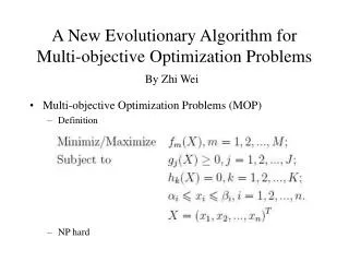
4. Single Objective Optimization Given: a functionf : A→R from some setA to the real numbers Sought: an element x0 in A such that f(x0) ≤ f(x) for all x in A ("minimization") or such that f(x0) ≥ f(x) for all x in A ("maximization").

5. Algorithms for Single Objective Optimization Gradient descent aka steepest descent or steepest ascent Hill climbing Simulated annealing Quantum annealing Tabu search Beam search Genetic algorithms Ant colony optimization Evolution strategy Stochastic tunneling Differential evolution Particle swarm optimization Harmony search Bees algorithm Dynamic relaxation

6. Multi-Objective Optimization 6 Courtesy of Dr. YoaChu Jin

7. Multi-Objective Optimization 7 m= 1 , single objective optimization Courtesy of Dr. YoaChu Jin

8. 8 Solutions for Multi-objective Optimization • Map into a single objective optimization by a weighted sum • The multi-objective approach (rank-based fitness assignment method) to evaluate each objective individually

9. Comparison of the single objective approach and the multi-objective approach • SO • + simple • - Hard to determine weight for each objective . • Hard to prevent some objectives from dominating others. • MO • + Have the ideal situation where each objective function attains a satisfactory level. • + Have the flexibility to achieve different levels of tradeoff. • - Not so easy to solve.

10. Single GA

11. Single GA Parent A 110011001 Parent B 101111011 110011001 …. …. 101010101 110011001 101111011 …. 101010101 110011001 => 110101001 110011001 110011011 101111011 101111001 110011001 101111011 …. 101010101

12. Pareto Front proximity Introduction of multi-objective genetic algorithm Task 1: To find a set of solutions as close as possible to the Pareto-optimal front. Task 2: To find a set of solutions as diverse as possible f2 Solution Space Dominated solutions Nondominated solutions Diversity f1  Minimization Objective 1

13. The variable length genetic algorithm • Why Variable-Length GAs (VLGAs)? • The number of solutions is not fixed. • i.e. Fixed Length GAs must know number of variables a priori • Ex: Finding number of base stations for • a given region • Ex: Finding rules for autonomous agents

14. Evolutionary of the variable length multi-objective optimization • The number of solutions is not fixed. • It is a multi-objective optimization problem • We would like to solve the problem by GA

15. Pareto Front proximity Evolutionary of the variable length multi-objective optimization Nondominated solutions f2 Solution Space Dominated solutions Nondominated solutions Diversity f1  Minimization Objective 1

16. Evolutionary of the variable length multi-objective optimization Rank-based fitness assignment method f2 3 3 5 1 8 3 Front 4 1 5 Front 3 2 4 Front 2 1 Front 1 1 1 1 f1

17. Evolutionary of the variable length multi-objective optimization

18. Applications MOGA - Aircraft routing VLMOGA - Placement of heterogeneous wireless transmitters

19. Application 1 Aircraft Routing using Multi-objective Genetic Algorithm

20. Problem Description • Aircraft routing • A given set of flights  a group of aircrafts • Available amount of aircrafts

21. Aircraft Routing (1/2) Timetable  assign to aircrafts

22. Aircraft Routing (2/2) f2 f3 f9 f6 f10 f4 f17 f1 f12 f19 f14 f5 f7 f18 f11 f20 f8 f15 f16 f13 Flight set F aircraft 1 f8 f2 f13 f11 aircraft 2 f3 f6 f4 f10 f17 aircraft 3 f18 f16 f19 f9 f5 f15 Flight schedule S aircraft 4 f20 f1 f14 f7 f12

23. Notations • Let α, β, ω, andγ represent • α: number of aircrafts • β: maximal number of flights per aircraft • ω: number of airports • γ: number of daily flights, respectively. • Set of flights: F ={fi|1 ≤ i ≤ γ} • Set of airports: P = {pj|1 ≤j ≤ ω} P= {台北松山機場、 高雄小港、 台中、 台南 、馬公、 金門}

24. , Associate Information of One Flight The flight schedule S can be represented as: si,j:the jth flight assigned to the ithaircraft : origin of si,j, where : destination of si,j, where : departure time from : arrival time in

25. Definition of a Flight Schedule Maximal flights assigned to each aircraft Number of aircrafts

26. Flight Schedule S Number of aircrafts Maximal flights assigned to each aircraft s1,1 sα,β

27. Objectives • Objectives: • Ground turn-around time objective • Flow balance objective Subject to

28. Ground Turn-around Objective(1) Legal ground turn-around time: TGH

29. Flow Balance Objective(2) Extra cost

30. Encoding Scheme

31. Crossover

32. Reciprocal Mutation A B C D E F A B E D C F

33. Experimental Results • 7 airports, 9 aircrafts, 12 flights one day, 79 flights.

34. Experimental Results

35. Symbols in Experimental Results Gantt chart: time Aircraft1/crew1 Aircraft2/crew2 departure time flight ID 682 KNH TSA origin destination arrival time

36. Scheduling Result of 9 aircrafts

37. Scheduling Result of 8 aircrafts Example ε = [ε1, ε2] =[k1 × α× TGH, k2× α] = [1 × 8 × 25, 1 × 8] = [200, 8]

38. Scheduling Result of 8 aircrafts Result1 Result2 Result3

39. Scheduling Result of 8 Aircrafts

40. Retiming Process Flights P and Q can beassigned to the same aircraft Flights P and Q cannot beassigned to the same aircraft

41. Scheduling Result-Retiming

42. Application 2: Heterogeneous Wireless Transmitter Placement with Multiple Constraints based on the Variable-Length Multi-objective Genetic Algorithm

43. Problem statement Choose a set of heterogeneous wireless transmitters to place on the designed space to fulfill certain design requirements such as Position, power, capacity, frequency channel assignment, overlap, data rate demand, population density, cost and coverage Evolutionary multiobjective optimization for base station transmitter placement with frequency assignment, IEEE Trans. on Evolutionary Computation, 2003

44. Introduction (cont.) 23meters 15meters

45. Parameters

46. Wireless transmitter placement problem

47. Problem Definition • Model • Map, receiver, transmitter • Receiver • Position, data rate demand, sensitivity • Transmitter • Position, type=(cost, power, capacity)

48. Path Loss Propagation Models • Free space path loss model • Log-distance path loss model with shadowing effect • ECC-33 model

49. Objectives • Coverage • Cost • Data Rate Demand • Overlap

50. Coverage Coverage Rate=4/9=44.4% Uncoverage=5