Pre-Main Sequence evolutionary models (low and intermediate mass)
Pre-Main Sequence evolutionary models (low and intermediate mass). Scilla Degl’Innocenti Emanuele Tognelli Pier Giorgio Prada Moroni ( Physics Department , Pisa University ).

Pre-Main Sequence evolutionary models (low and intermediate mass)
E N D
Presentation Transcript
Pre-MainSequenceevolutionarymodels(low and intermediate mass) Scilla Degl’Innocenti Emanuele Tognelli Pier Giorgio Prada Moroni (PhysicsDepartment, Pisa University)
Huge amount of observational data in young clusters and star forming regions in the Milky Way and Magellanic Clouds (Jeffries et al. 2014, Alcalà et al. 2014, Patience et al. 2014, Bouy et al. 2014, Sarro et al. 2014, Sacco et al. 2014, Robberto et al. 2013, Manara et al. 2013, Lopez-Marti et al. 2013, Spezziet al. 2012, Alves De Oliveira et al. 2012, Bayo et al. 2012, Scandariato et al. 2012, Da Rio et al. 2012, Gougliermis et al. 2012, D’Orazi et al. 2009, Luhman et al. 2009, 2008, Enoch et al. 2009, Cignoni et al. 2010, Brandner et al. 2008, Reipurtet al. 2008 and references therein). To infer the star formation rate and initial mass function updated Pre-MS evolutionary models are mandatory Pisa Pre-MS models
Several Pre-Main Sequence database available in the literature (see e.g. Lagarde et al. 2012,Tognelli et al. 2011, Di Criscienzo et al. 2009, Dotter et al. 2008, Yi et al. 2001, Siess et al. 2000, Charbonnel et al. 1999, Palla & Stahler 1999, Baraffe et al. 1998, D’Antona & Mazzitelli 1997…) The interpretation of a direct comparison among different evolutionary database is not so easy! (see e.g. Tognelli, Prada Moroni, Degl’Innocenti 2011, Hillebrand et al. 2008, Hillebrand and White 2004, etc..) Quantitative analysis of the effects of uncertainties affecting both standard (no rotation, no magnetic fields, no mass loss etc..) and non standard PMS models
The adoption of a grey T(t) relationship is a too crude approximation for the integration of cold atmospheres (see e.g. discussions in Auman 1969, Dorman et al. 1989, Saumon et al. 1994, Baraffe et al. 1995, Allard et al. 1997, Chabrier & Baraffe 1997, Baraffe et al. 1998, 2000) Thus all the evolutionary models are made with boundary conditions obtained from atmospheric models: P(tph,Teff, g, [Fe/H]) and T(tph,Teff, g, [Fe/H]) at tphprovidedbydetailed, non-greyatmosphericmodelswhich solve the full radiative transportequation -BH05(default, Brott & Hauschildt 2005): 2000 K ≤ Teff ≤ 10 000 K; -CK03(Castelli & Kurucz 2003): Teff > 10 000 K; - AHF11 (Allard et al. 2011): Teff < 2000 Boundary conditions at the bottom of the atmosphere
Chemical composition determination (metallicity, helium abundance, mixture..) Adopted physical inputs Main sources of uncertainty on theoretical predictions (EOS, opacity, nuclear reaction rates..) Physical mechanisms (diffusion, external convection efficiency, boundary conditions..) Main sources of uncertainty for the position of tracks and isochrones in the HR diagram
Chemical composition uncertainties Uncertainties on [Fe/H], Z and Y From [Fe/H] by adopting a solar scaled mixture one obtains the helium abundance Yand the total metallicity Z Dlog L/Lsun ≈ 0.01 – 0.1 (see e.g. Pagel & Portinari 1998 ) • By assuming: • - D[Fe/H] ≈ ±0.01, ±0.1 (we adopts ±0.05); • - DYP ≈ 0.2485 ±0.008 (Cyburt 2004); • - DY/DZ ≈ 2 ± 1 (Casagrandeet al. 2007); • -D(Z/X)sun≈ +25/-10 % (see discussion in Tognelliet al. 2012) • Large differences in Teff in all the models both along the Hayashi track and in ZAMS • Luminosity is significantly affected only in not fully convective models DTeff ≈ 50 – 100 K DTeff ≈ 200 – 400 K DTeff ≈ 50 – 100 K Reference values (Y=0.274, Z=0.01291, [Fe/H]=0) (Tognelli et al. 2011)
Warning Whencomparing data with theoreticalpre-MStracks, one must use models with the samemetallicity of the observedstars Anchangein [Fe/H] betweenobservations and modelstranslatesin a shift in Teff/L and hence in an error in theinferred mass and age Δ[Fe/H]=0.2 dexleads to a shift in Teffof≈100 K ΔM=0.1 Mo Δt≈70 %
Chemical composition uncertainties Solar mixture In PMS models solar mixture (at fixed Z) affects opacity: Atmosphere. Molecules (CO, H2O, TiO) for logT(K) < 3.8 (Ferguson et al. 2005) Interior. Hydrogen and metals: log T(K) = 5.2 – 5.8, e 6.4 – 6.8 iron group elements Fe (Cr, Fe, Ni) (Iglesias & Rogers 1996, Sestito et al. 2006) Widely adopted solar mixtures -GN93(Grevesse & Noels 1993); -GS98(Grevesse & Sauval 1998); - AS05(Asplund et al. 2005); -AS09(Asplund et al. 2009); (see also mixture evaluations by Caffau et al. 2010, Pereira et al. 2009, Grevesse et al. 2007)
Chemical composition uncertainties Solar mixture DTeff ≈ 90 – 100 K DTeff ≈ 200 – 350 K Models with radiative cores are sensitive to a mixture variation (at fixed Z) (Models with Asplund et al. 2009 and Asplund et al. 2005 mixtures are very similar)
Physical inputs uncertainties Equation of state (EOS) EOS plays a crucialrole, in particular in the convectiveregionsof low mass stars, which are almostadiabatic(see e.g. Mazzitelli 1989, D’Antona 1993 and referencestherein) Teff and Roflow-massstars are determinedby the adiabaticgradient, i.e. EOS Effects of adopting different EOS*: For PMS stars with M < 1.0 Msun : maximumDTeff≈ 50 - 70 K If updated EOS are adopted the residual uncertainties do not affect in a relevant way the evolution in the HR diagram *(PTEH95= Pols et al. 1995, FreeEOS08, see Irwin et al. 2004, SCVH95=Saumon et al. 1995, OPAL 2006,2001 see Rogers et al. 1996, Rogers & Nayfonov 2002) (Tognelli et al. 2011)
Physical input uncertainties 14N(p,g)15O cross section S(0)=1.57 ± 0.13 KeV-b (LUNA collaboration, see e.g. Formicola et al. 2003, Marta et al. 2008 and references therein) DTeff ≈ 350K DTeff ≈ 40 K DTeff ≈ 250 K M≥ 1.5 Msun are affected starting from ZAMS (Tognelli et al. 2011, see also Straniero et al. 2002, Imbriani et al. 2004, Degl’Innocenti et al. 2004, Weiss et al. 2005)
Uncertainty on convection efficiency* A widelyusedapproachis the mixing length theory** (Bohm-Vitense 1968) , in which the averageconvectiveefficiencydepends on the freeparametera, tobecalibratedwithobservations The usualapproachis the solarcalibrationwhich, however, doesnotrely on a physicalargument, sincethereis no reasontoexpectthat the efficiencyofconvectionis the sameforstarsofdifferentmasses and differentchemicalcompositions(see e.g. Canuto & Mazzitelli 1992, D’Antona & Mazzitelli 1994, 1998, Montalbanet al. 2004) Moreoverthereis no reasonto assume a constanta valuealong the wholeevolutionof a star(see e.g. Siess & Livio 1997, Ludwig et al. 1999, Trampedachet al. 1999, 2007, Montalban & D’Antona 2006) *Discussed by several authors, see e.g. Petersen 1990, Canuto & Mazzitelli 1992, D’Antona 1993, D’Antona & Mazzitelli 1994, 1997, Salaris & Cassisi 1996, Baraffe et al. 2000, D’Antona & Montàlban 2004, Montàlban et al. 2004, Landin et al. 2006 ** Some evolutionary codes adopts the Full Spectrum Turbulent convection treatment (see e.g. Canuto & Mazzitelli 1991, Canuto et al. 1996)
Uncertainty on convection efficiency The assumedconvectionefficiencyisrelatedto the uncertainty on otherinputswhichaffect the effective temperature Itispossible to obtainmanysolar models with significantlydifferentpre-MSlocations and shapes(see e.g. D’Antona & Mazzitelli 1994, Montalbanet al. 2004) DTeff 50 K SSM (Tognelli, Prada Moroni, Degl’Innocenti 2011) At present, arepresentsanuncertainty source
Uncertainty on convection efficiency Dependence on a: DTeffuntil 500 K - M < 0.2 – 0.1 Msun: mild dependence: almost adiabatic stars - 0.2 Msun < M < 0.6 Msun: dependence only along the Hayashi track . - 0.6 Msun < M < 1.2 Msun: dependencealong the wholepre-MS - M > 1.2 Msun: dependenceonlyalong the Hayashitrack
Uncertainty on convection efficiency The uncertainty on aMLalsoaffectsboth mass and ageestimatesofyoungstarsifobtainedthrough the comparisonof the stellar position in the HR diagram (Tognelli, Prada Moroni, Degl’Innocenti 2011) The greatestdifferenceoccursnear the Hayashitrack
Uncertaintes: matchingpointbetweeninterior and atmosphere The value of tph, the optical depth at which interior and atmosphere matches must be chosen in a way that: - enough large to guarantee photon diffusion approximation; - enough small to reduce discrepancies due to inconsistencies between atmospheric and interior models . generally: tph: 2/3 ÷100 (see e. g Montàlbanet al. 2004, Tognelli et al. 2011) DTeff ≈ 90 K Main effects on cold objects: low mass stars and Hayashi track Reference value: tph= 10 (see e. g. Morel et al. 1994)
Modeluncertainties: conclusions PMS models (extremely) sensitive to: originalchemicalcomposition, EOS, convectionefficiency, atmospheric treatment The adoptionofupdatedevolutionarymodelsfor the comparison withobservationsismandatory
Pisa pre-MS database • Very fine grid of masses and chemical compositions • 11653 tracksand 10080 isochrones. • - 43stellar mass values, 0.2 ÷ 7.0 Msun • - 20metallicities(Z); • - 3original helium abundances (Y); • - 2original deuterium abundances (Xd); • 3 mixing length values (aML). • Isochrone ages: 1 – 100 Myrfor each set (Tognelli, Prada Moroni, Degl’Innocenti 2011) Standard solar model: Y=0.253, Z=0.0138, a=1.68 Xd=2 . 10-5
The database is available at the URL: http://astro.df.unipi.it/stellar-models/
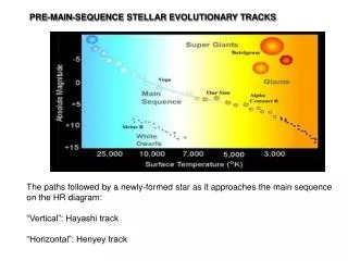
Uncertainties on the initialconditions The very common procedureofstarting PMS evolutionfrom a model on the Hayashitrackwith a largeradius and luminositydefiningitas “the zero agemodel” isnot, in principle, a realistic procedurebecauseitneglects the protostellarphase(see e.g. Stahler 1980, 1983, Hartmannet al. 1997) However…IFwebelievethatonce the mainaccretionphaseisfinished, the evolutionquicklyconvergestothatof standard hydrostaticmodels(see e.g. Stahler 1983, Palla & Stahler 1999)… ..in this caseone can analyse the effectsofstartingfromdifferentpointsalong the Hayashitrack. Modelsshould start from thebirth linedefinedas the locus in the HR diagramwhere the star endsitsaccretionphase(Stahler 1983)
Under thesehypothesisbirthlineislocated in the regionof the HR diagramcorrespondingtolarge and brightstructures
The structurelosesmemoryofthisinitialmodel and whenthisoccurs? Thatisagesinferredforveryyoungstars are reliable? “Zero AgeModel” : expansestructurewithTc = 1÷2 105 K no deuteriumburning IfTc ≤ 3.5 105 K the tracks converge to an uniquesolutionbefore 1 Myr (Seealsodiscussions in Baraffeet al. 2000, D’Antona & Montalban 2006, Landinet al. 2006, Scandariatoet al. 2012)
Does the accretionphaseaffects PMS evolution? • Starsformfrom the fragmentationsofmolecularclouds, whichprovide the seedsof future stars (protostars). Then the remaining mass isaccretedduringconstant and/or timedependentaccretionepisodes. • Despiteof the hugeobservationaleffort* the accretiongeometry (disk or spherical), the accretion rate and itstimedependence, the mass and radiusof the initialprotostellarseed are stilluncertain • Regardingprotostellarevolution**: 1) sphericalapproach(proposed by Stahler et al. 1980, seealso 1981, 1986, Palla & Stahler 1991) 2) disk accretionmodel(proposedbyHartmannet al. 1997 and Siess & Livio 1997) • The evolutionof the protostarisstronglydependent on the accretionparameters, mainly on the fractionof the accretionenergydeposed inside the star. • *See e.g. Hartiganet al. 1991, Hartmannet al. 1998, 2011, Hillenbrandet al. 1998, Ladaet al. 2000, 2001, Haischet al. 2001, Calvetet al. 2004, Allerset al. 2006, Ladaet al. 2006, Luhmanet al. 2008,2012, Flaherty & Muzerolle 2008, Enochet al. 2009, Hernandezet al. 2010, Rigliacoet al. 2011, Spezzi et al. 2012, Manara et al. 2012, Ercolano et al. 2014, Alcalàet al. 2014, Dunhamet al. 2014 and referencestherein. • ** FormodelsofaccretingstarsseealsoBehernd & Maeder 2001, Yorke & Sonnhalter 2002, Baraffeet al. 2009, 2012, Baraffe & Chabrier 2010, Hosokawaet al. 2010, 2011, Haemmerléet al. 2013 • Forhydrodinamicalsimulationsofcollapsingclouds, seeMasunagaet al. 1998, Masunaga & Inutsuka 2000, BoyodWhitwort 2005, Vorobyov & Basu 2005,2006, 2010, Machidaet al. 2010, Tomidaet al. 2010, 2013, Dunham & Vorobyov 2012 and referencestherein
Non standard PMS models The ’’classicaltheory’’ of stellar evolution(sphericalsymmetry, no effects of rotation, mass loss, magneticfields and so on)fails to explainnearlyallobserved Li and Be surfaceabundancepatterns Several non standard modelswasproposed* (rotationalinduced mixing, travelinginternalgravitywaves, tachocline, a combination of gravitywaves and rotation, internalmagneticfields, mass lossetc ..) However the effects on L, Teff and evolutionary time of PMS modelsisquitenegligible(see e.g. Charbonnel et al. 2013, Eggenberget et al. 2012, Landin et al. 2006), butformodelswhich assume a variationofTeff and radius due to the presenceof strong magneticfields *ReviewsbyPinsonneault 1997, Delyannis 2000, Jeffries 2000, 2006, Pasquini 2000, Charbonnel 2000, Siess 2000, Randich 2006. SeealsoZahn (1984), 1992, Michaud (1986), Pinsonneault et al. 1989, 1992, Charbonneau & Michaud 1991, Garcia Lopez & Spruit1991, Chaboyer & Zahn 1991, Charbonneau 1992, Spergel & Zahn 1992,Schatzman 1993, Deliyannis & Pinsonneault 1997, Mendez et al. 1997, 1999, Zahn et al. 1997, Kumar & Quataert 1997, Gough & Mac Intire 1998, Maeder & Zahn 1998, Talon & Charbonnel 1999, Charbonnel & Talon 1999, 2005, Brun et al. 1999, Montalban & Schatzmann 2000, Talon et al. 2002, Piau et al. 2003, Michaud et al. 2004, Landin et al. 2006, Eggenber et al. 2008, Pace et al. 2012, Lagarde et al. 2012, Eggenberger et al. 2012, Charbonnel et al. 2013
Observational test: binarysystems* Few (27) PMS starswithdirect mass measurements(see e.g. Mathieuet al. 2007, Stempelset al. 2008, Cusanoet al. 2010) Comparisonmadebymeansof a Bayesianmethod(byJorgensen & Lindegren 2005) (Gennaro, Prada Moroni, Tognelli 2010) *see e.g. Simon et al. 2000, Steffenet al. 2001, Hillebrand & White 2004, Stassunet al. 2004, Mathieuet al. 2007, Badenet al. 2007, Alecianet al. 2007, Stassun 2008, Jackson et al. 2009, Torres et al. 2010, Feiden & Chaboyer 2012 and referencestherein
Observational test: binary systems • In agreement with previous results: • For standard models masses tend to underestimated, however • (Gennaro, Prada Moroni, Tognelli 2010) • in the case of double line eclipsing • binary systems the agreement is • quite good (maximum relative differences • 15% - 20% and in some cases differences as • small as 5%, but V1174 Ori) • Regarding the age the situation is • slightly worse (30% of the systems result • not coeval) • Suggestions for the preference for colder models (low external convection efficiency, a=1 ?) in agreement with previous results (see e.g. D’Antona et al. 2000, Simon et al. 2001, Steffen et al. 2001, Baraffe et al. 2002, D’Antona & Montalban 2003, Stassun et al. 2004, Covino et al. 2004, Claret 2006, Alves de Oliveira 2013) fuori 2-sigma fuori 2-sigma Link (?) with the underestimate of radii in PMS binary systems noticed by several authors (see e.g. Stassun et al. 2006, 2007, Mathieu et al. 2007, Jackson et al. 2009, Torres et al. 2010, Feiden & Chaboyer 2012, Somers & Pinsonneault 2014)
Lithium abundance in PMS stars Why lithium is so important? • It is a fragile element destroyed through proton capture at relatively low • temperature, i.e. T ≈ 2.5 million degrees, easily reached even during the • early pre-MS evolution; • It is only destroyed in PMS stars: lithium surface abundance depends only • on the initial amount of lithium present in the star and on the efficiency of • the depletion processes; • Lithium is a very good tracer of both the efficiency of the mixing • processes present in the star and the temperature stratification. It • gives precious information about thestructure of the convective envelope • ( see e.g. reviews in Delyanniset al. 2000, Jeffries 2000, Pinsonneaultet al. 2000, Charbonnelet al. 2000, Talon 2008, Talon & Charbonnel 2010, Jeffries 2006…)
General features of Lithium burning in pre-MS 2 1- Onset of lithium burning: Fully convective star. 2 - Formation of a radiative core: Lithium burning still possible at the base of the convective envelope if TCE ≥ TLi . 3 - The extension of the convective envelope reduces: TCE decreases, lithium burning is halted. 3 1 3 PMS 7Li surface depletion strongly depends on the mass and on the metallicity of the star
General features of Lithium burning in pre-MS Lithium pre-MS depletion is extremely sensitive to the convection efficiency - Mixing Length Theory (Bohm-Vitense1968) Introduction of the free parameter α(lc = αHP) - Calibration of α: Sun, CMDs for main- sequence stars. Standard models fail in reproducing the observed 7Li abundances in young clusters if a solar/MS convection efficiencyis assumed in PMS hints for a reduced convection efficiency (see e.g. D’Antona & Mazzitelli 1994, 1997, Ventura et al. 1998, Schlatt & Weiss 1999, Piau & Turck-Chièze 2002, D’Antona & Montalban 2003, Landin et al. 2006, Eggenberger et al. 2012, Tognelli et al. 2012, Sommers & Pinsonneualt 2014 and references therein )
Uncertainties on predictedsurfacelithiumabundance* • Chemical composition • Uncertainties on YP,(Z/X), [Fe/H], ΔY/ΔZ, solar mixture - Physical Inputs Opacity coefficients(radiative opacity): uncertainty of about± 5%from differences between OPAL 2005 (see e.g. Iglesias & Rogers 1996) and OP (Seaton et al. 1994, Badnell et al. 2005), see also Neuforge-Verheecke et al. 2001, Bahcall et al. 2005, Badnell et al. 2005, Valle et al. 2012). 7Li +preaction Rates: uncertainty about± 5% (Lattuada et al. 2001; Pizzone et al. 2003). EOS:uncertainties evaluated by comparing the results obtained from several EOS widely used in the literature (OPAL2001, SCVH95, PTEH) Initial D and 7Li values : XD= 2 . 10-5(see e.g. Geiss & Gloeckler 1998, Linsky et al. 2006, Steigmann et al. 2007) A(Li) = log NLi/NH + 12 = 3.2 ± 0.2 (see e.g. Jeffries 2006, Lodders et al. 2009) * See alsoMazzitelli 1989, D’antona 1993, Swenson et al. 1994, D’Antona & Mazzitelli 1994, Chabrier & Baraffe 1997, Piau & Turck-Chièze 2002, D’Antona & Montalban 2003, Landin et al. 2006, Sestito et al. 2006, Tognelli et al. 2011, Somers & Pinsonneault 2012 and references therein
Uncertainties on predictedsurfacelithiumabundance Error bars: we quadratically added the differences in surface lithium abundances and effective temperature obtained taking into account the quoted error sources The uncertainties on the chemical composition, physical inputshave astrong effect on the predictions of surface lithium abundance in particular for low-mass stars chemical composition physical inputs Tognelli, Degl’Innocenti, Prada Moroni 2012
Comparison with selected young open clusters Open clusters: Ic 2602, α Per, Blanco 1, Pleiades, Ngc 2516 30-40 Myr< age< 130-150 Myr -0.10 ≤ [Fe/H] ≤ +0.07 Colour-Magnitude Diagram :high quality photometric observations (HIPPARCOS when available) Lithium data by Sestito& Randich (2005) Large homogeneous database of observational data for surface 7Li abundance in open clusters of different ages and chemical compositions
Comparison with selected open clusters The method Isochrone fitting: determine the “best value” of the ageand of the mixing lengthparameter for MS stars (αMS) with the related errors Uncertainty on age determination: 10-20 Myr, mainly from the lack of stars near the overall contraction region Not negligible for mid- and low-mass stars in cluster younger than about 60-70 Myr, completely negligible in the other cases Consistency: the models adopted for surface lithium predictions are the same as the ones adopted for the isochrone fitting
Comparison with selected open clusters Lithium predictions Standard models + models in which we allow different values of αduring pre-MSand MS evolution - Additional physical mechanisms not taken into account in standard PMS models - Hints of non-constancy of αfor stars in different masses and evolutionary phases from observations (see e.gChieffi et al. 1995, Morel et al. 2000, Ferraro et al. 2006, Yildiz 2007, Gennaro et al. 2012, Piau et al. 2011, Bonaca et al. 2012) and detailed hydrodinamical simulations (e.g. Ludwig et al. 1999; Trampedach 2000) • one chooses the best value of αPMSto reproduce the observed surface 7Li • abundance in each cluster; • αMSis constrained by the comparison with the Colour-Magnitude Diagram.
60 Myr 40 Myr 120 Myr Ages are in quite good agreement with previous determinations 110 Myr 130 Myr Tognelli et al. 2012
Previousindicationsfor a low PMS convectionefficiency are confirmed* • It’s possible to reproducethe observed 7Li(Teff) profile by adopting the same αPMSfor all the selected clusters (independence of pre-MS mixing lengthparameter on the chemical composition and age for clusters younger than about 150-200 Myr) • Clearlyit’s notpossibletoreproduce the spread in Li abundance forcoolstars (Teff≤ 5500K) observed in some youngclusters (e.g. Pleiades) 1.30 M 1.00 M 1.00 M 1.00 M 1.20 M 0.70 M 0.65 M 0.60 M αPMS = 1.0 *See e.g. Ventura et al. 1998; Simon et al. 2000; Steffen et al. 2001; D’Antona & Montalban 2003; Stassun et al. 2004, Landin et al. 2006, Somers & Pinsonneault 2014 1.40 M 1.00 M 1.00 M 0.70 M 0.65 M (Tognelli et al. 2012)
???? • Rotating models (with or without gravity waves) provide (slightly) higher Li depletion especially for low mass stars rotation alone cannot solve the problem (see e.g. Pinsonneault et al. 1989, Martin & Claret 1996, Mendes et al. 1999, Landin et al. 2006, Eggenberger et al. 2012, Chaboyer et al. 2013) • Several possible solutions of the problem(s): • Rotation + star disk coupling + low convection efficiency ( see e.g. Eggenberger et al. 2012) • inhibition of convection by magnetic activity ( see e.g. Ventura et al. 1998, Mullan & Mac Donald 2001, D’Antona & Montalban 2003, Landin et al. 2006, Chabrier et al. 2007, Morales et al. 2008, 2010, Mac Donald & Mullan 2012, Feiden & Chaboyer 2013, Somers & Pinsonneault 2014) • Effects of accretion history (see e.g. Baraffe & Chabrier 2010) • Li dispersion is (at least in part) spurious : stellar surface activity, wrong temperature scale, inhomogeneous reddening, rotational broadening of Li absorption lines in rapid rotators ( see e.g. Luhman et al. 1997, King et al. 2000, Margheim et al. 2002, Hillenbrand & White 2004, Pace et al. 2012 ) • Comparisons with binary stars with dinamical mass and 7Li abundance values (ASAS J052821, EK Cep, RXJ 0529, V1174 Ori) cannot help to discriminate between low and high convection efficiency due to the still large observational errors (Tognelli et al. 2012, see also D’Antona & Montalban for RXJ 0529)
Even more precise observational data are needed: • masses, radii, rotation velocities, lithium abundances, magnetic activity • for PMS binary stars • effective temperatures, rotation velocities, magnetic activity, accretion • rates, lithium abundances for young clusters and star forming regions • …… • …in a way to constrain the large amount of models that we, as theoreticians, • have fun to produce!
- Evolutionary Code: FRANEC Updated physical inputs (see Tognelli et al. 2011) Equation of State: OPAL EOS 2006 (Rogers & Nayfonov 2002); Radiative Opacity: OPAL 2005 (Iglesias & Rogers 1996)for log T[K] > 4.5, Ferguson et al. (2005)for log T[K] ≤ 4.5; Heavy Elements Solar Distribution: Asplund et al. (2005); Boundary Conditions: Brott & Hauschidt (2005) for T < 10 000 K and Castelli & Kurucz (2003) for T ≥ 10 000 K. Match between atmosphere and interior computations at the optical depthτph = 10;
Uncertainties on theoretical predictions • Chemical composition of the star. • From the observations we obtained [Fe/H] (spectroscopic). Helium and metals abundance (Y, Z) are compute using the relation: • for solar-scaled metal distributionplus a linear relation between helium and metal abundance. (YP : primordial helium abundance. (Z/X) : photospheric metal-to-hydrogen ratio • abundance in the Sun. ΔY/ΔZ : helium-to-metal enrichment ratio.) • Uncertainties onYP,(Z/X),[Fe/H] andΔY/ΔZ propagate into uncertainties on YandZ. plus • Typical uncertainties on such quantities: • Δ[Fe/H] ≈ ± 0.05 dex • Δ(Z/X)/(Z/X) ≈ 15% (Bahcall et al. 2005) • YP = 0.2485 ± 0.0008 (Steigman 2006) • 1 ≤ ΔY/ΔZ ≤ 5 (see e.g. Gennaro et al. 2010) • εLi-7 = 3.2 ± 0.2 (see e.g. Lodders 2009) A change in YandZ affects the structure of the star hence lithium depletion
Physical inputs uncertainties EOS For PMS stars the temporal evolution of the luminosity is slightly dependent on the EOS with a maximum difference for the ZAMS age of ≈ 20% while, except for M≤ 0.1 Msun , Dlog L/Lsun ≤ 0.02 PMS isochrones If updated EOS are adopted the residual uncertainties does not affect in a relevant way the evolution in the HR diagram (Tognelli et al. 2011)
CNO cross sections and cluster ages The cross section update influencesonly the agedetermination for old clusters (see Straniero et al. 2002, Imbriani et al. 2004, Degl’Innocenti et al. 2004, Weiss et al. 2005) L3αHB (14N+p) LTO McHe LCNOHB * For (14N+p)/2 ΔLogLHB~0.01 (Z=0.0002) * For (14N+p)/2 ΔLogLHB~ -0.01 (Z=0.001) Maximum age variation by adopting the vertical method ~ 1 Gyr Degl’Innocenti et al. 2004
Cosmological D abundance: 3.8x10⁻⁵ ≤ XD ≤ 4.5x10⁻⁵ (Cyburt et al. 2004, Steigman et al. 2007, Pettini et al. 2008) As stellar generations follow each other, D is astrated, since stars are net destroyers of D Solar neighbourhood D abundance: XD ≈ 2.5-3x10⁻⁵ (Geiss & Gloeckler 1998, Vidal-Madjar et al. 1998, Linsky 1998, Linsky et al. 2007, Steigman et al. 2007) Pisa Models: D-burning
Deuterium abundance: D is destroyed at about 106 K (early pre-MS). p(d, 3He)g Q = 5.493 MeV(Qpp ≈ 26 MeV) Temporarily halts gravitational constraction Contrazione gravitazionale: riparte quando Xd ≈ 1/100 valore iniziale
The value of XD affects only the very early evolution After a few Myr the isochrones converge XD= 4x10⁻⁵ for all stars XD= 2x10⁻⁵ for Z>0.007 Pisa Models: D-burning
Pisa Solar Model Other standard solar models
Atmosferestellariimplementate: Atmosferenon-grigie(tabellemodelliteoricidettagliati, ideali per M < 1 Msun). -BH05(default, Brott & Haushildt 2005): 2000 K ≤ Teff ≤ 10 000 K; -CK03(Castelli & Kurucz 2003): Teff > 10 000 K; - AHF11 (Allard et al. 2011): per stelledipiccolamassaTeff < 2000 K; Atmosferegrigie(modellisemplificati, M ≥ 1 Msun). -KS66(Krishna-Swamy 1966) Effetto su strutture con inviluppi convettivi! DTeff ≈ 100,(max > 200 K) DTeff ≈ 100 - 150 K DTeff ≈ 100 - 200 K
Comparison with other authors Tognelli, Prada Moroni & Degl’Innocenti2011