Compensating wage differentials
Compensating wage differentials . Heterogeneity. One limitation of the static LS model lies in the heterogeneity assumption. In reality, individuals differ in preference and in information acquired. We thus need to have such heterogeneity in the model . Household production.

Compensating wage differentials
E N D
Presentation Transcript
Heterogeneity • One limitation of the static LS model lies in the heterogeneity assumption. • In reality, individuals differ in preference and in information acquired. • We thus need to have such heterogeneity in the model
Household production • Suppose several unskilled workers have received offers from two employers. • Employer X pays $8 per hour and offers clean, safe working conditions. Employer Y also pays $8 per hour but offers employment in a dirty, noisy factory. Which employer would the workers choose? • Clearly, however, $8 is not an equilibrium wage in both firms. Because firm Y must pay a wage above $8 to be competitive in the labor market. The extra wage it must pay to attract workers is called a compensating wage differential.
Hedonic wage theory • In economics, hedonic regression or hedonic demand theory is a revealed preference method of estimating demand or value. • It decomposes the item being researched into its constituent characteristics, and obtains estimates of the contributory value of each characteristic. • Here, we analyze the theory of compensating wage differentials for a negative job characteristic, the risk of injury. • Applying the concepts to a normative analysis of governmental safety regulations.
Representative Indifference Curves for Two Workers Who Differ in Their Aversion to Risk of Injury
Two workers • The more-sensitive workers will have indifference curves that are steeper at any level of risk • The slope at point C is steeper than at point D. • Point C lies on the indifference curve of worker A, who is highly sensitive to risk, while point D lies on an indifference curve of worker B, who is less sensitive.
Firms • Employers are faced with a wage/risk trade-off of their own that derives from three assumptions. • It is presumably costly to reduce the risk of injury facing employees. • Competitive pressures will presumably force many firms to operate at zero profit(that is, at a point at which all costs are covered and the rate of return on capital is about what it is for similar investments). • All other job characteristics are presumably given or already determined. • The consequence of these three assumptions is that if a firm undertakes a program to reduce the risk of injury, it must reduce wages to remain competitive..
Two firms • Employers differ in the ease (cost) with which they can eliminate hazards. • The cost of reducing risk levels is reflected in the slope of the isoprofit curve. • In firms where injuries are costly to reduce, large wage reductions will be required to keep profits constant in the face of a safety program; the isoprofit curve in this case will be steeply.
Matching • Firm X, the firm that can cheaply reduce injuries, can make higher wage offers at low levels of risk (left of point R’) than can firm Y. • Because it can produce safety more cheaply, it can pay higher wages at low levels of risk and still remain competitive. • Any offers along segment XR’ will be preferred by employees to those along YR’ because, for given levels of risk, higher wages are paid.
Matching • At higher levels of risk, however, firm Y can outbid firm X for employees. Firm X does not save much money if it permits the risk level to rise above R, because risk reduction is so cheap. • Because firm Y does save itself a lot by operating at levels of risk beyond R, it is willing to pay relatively high wages at high risk levels. For employees, offers along R’Y’ will be preferable to those along R’X’, so those employees working at high-risk jobs will work for Y.
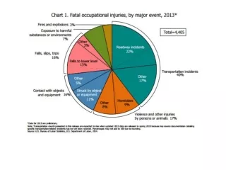
Example: parenthood and occupations • Men and women who are single parents choose to work in safer jobs. • Workers who are raising children feel a greater need to avoid risk on the job because they have loved ones who depend on them. • Men as single parents worked in safer jobs than married men, but married men with children apparently did not behave much differently than those without. Because married men are typically not in the role of caregiver to their children. • Married women, in contrast, do not find life insurance as effective in protecting children, because it provides only money, which cannot replace mother’s care.
The Effects of Government Regulation in a Perfectly Functioning Labor Market
Regulations under full information • Suppose workers are well informed about dangers inherent in any job and are mobile enough to avoid risks they do not wish to take. • In these circumstances, wages will be positively related to risk (other things equal), and workers will sort themselves into jobs according to their preferences. • Now, suppose the Department of Labor agency promulgates a standard that makes risk levels above RAX illegal. • For Y, reducing risk is costly, and the best wage offer a worker can obtain at risk RAX is WAX. • For B, however, wage WAX and risk RAX generate less utility than did Y’s offer of WBY and RBY.
Regulations under unbalanced information • A worker who believes she has taken a low-risk job when in fact she is exposing herself to a higher hazard. She receives a wage of W1 and believes she is at point J, while she is in fact at Kwith utility U0. • Now that the government discovers it and can pass a standard that limits employee exposure to this hazard. What level of protection should this standard offer? • Amandated risk level of R1would produce benefits that outweigh costs. That is, the amount that workers would be willing to pay (W1 – W*) would exceed the costs (W1 – W’’). A mandated risk levels between R0 and R2 would produce benefits greater than costs.
An Indifference Curve between Wages and Employee Benefits (payments in kind)
Flatter or steeper isoprofit curve • The trade-offs that employers are willing to make between wages and employee benefits are not always one-for-one. • Some benefits produce tax savings to employers when compared to paying workers in cash. • Workers with in-kind or deferred benefits instead of an equal amount of cash reduces their tax liabilities.