Understanding Differentials: Comparing Actual Change and Approximation in Calculus
This article delves into the concept of differentials in calculus, focusing on comparing actual changes (Δy) in a function to approximate changes (dy) derived from tangent lines. It illustrates the relationship between Δy and dy through step-by-step examples. One example explores the function y = 1 - 2x² at x = 1, demonstrating how to compute both changes when dx = -0.1. Another example considers the propagated error in the volume of a ball bearing, discussing how to estimate and interpret relative and percent errors in measurements.

Understanding Differentials: Comparing Actual Change and Approximation in Calculus
E N D
Presentation Transcript
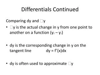
Differentials Continued Comparing dyand y • y is the actual change in y from one point to another on a function (y2 – y1) • dy is the corresponding change in y on the tangent line dy = f’(x)dx • dy is often used to approximate y
Given points P and Q on function f. The slope between P and Q is y / x The slope of the tangent line at P is dy/dx Notice: dx = xand dy ≈ y Q P
Example 1 Find both y and dy and compare. y = 1 – 2x2at x = 1 when x= dx = -.1 Solution: y = f(x + x) – f(x) = f(.9) – f(1) = -.62 – (-1) = .38 dy = f’(x)dx = (-4)(-.1) = .4 ** Note that y ≈ dy
Example 2 The radius of a ball bearing is measured to be .7 inches. If the measurement is correct to within .01 inch, estimate the propagated error in the volume V of the ball bearing. ** Propagated error means the resulting change, or error, in measurement
Example 2 Continued To decide whether the propagated error is small or large, it is best looked at relative to the measurement being calculated. • Find the relative error in volume of the ball bearing. ** Relative error is dy/y, or in this case dV/V • Find the percent error,(dV/V)*100.