Download
1 / 25
250 likes | 368 Vues
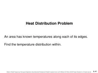
Heat Distribution Problem An area has known temperatures along each of its edges. Find the temperature distribution within. 6.41. Divide area into fine mesh of points, h i,j .

E N D
Heat Distribution Problem An area has known temperatures along each of its edges. Find the temperature distribution within. 6.41
Divide area into fine mesh of points, hi,j. Temperature at an inside point taken to be average of temperatures of four neighboring points. Convenient to describe edges by points. Temperature of each point by iterating the equation: (0 < i < n, 0 < j < n) for a fixed number of iterations or until the difference between iterations less than some very small amount. 6.42
Number points from 1 for convenience and include those representing the edges. Each point will then use the equation Could be written as a linear equation containing the unknowns xi-m, xi-1, xi+1, and xi+m: Notice: solving a (sparse) system Also solving Laplace’s equation. 6.45
Sequential Code Using a fixed number of iterations for (iteration = 0; iteration < limit; iteration++) { for (i = 1; i < n; i++) for (j = 1; j < n; j++) g[i][j] = 0.25*(h[i-1][j]+h[i+1][j]+h[i][j-1]+h[i][j+1]); for (i = 1; i < n; i++) /* update points */ for (j = 1; j < n; j++) h[i][j] = g[i][j]; } using original numbering system (n x n array). 6.46
Parallel Code With fixed number of iterations, Pi,j (except for the boundary points): Important to use send()s that do not block while waiting for recv()s; otherwise processes would deadlock, each waiting for a recv() before moving on - recv()s must be synchronous and wait for send()s. 6.48
Example A room has four walls and a fireplace. Temperature of wall is 20°C, and temperature of fireplace is 100°C. Write a parallel program using Jacobi iteration to compute the temperature inside the room and plot (preferably in color) temperature contours at 10°C intervals using Xlib calls or similar graphics calls as available on your system. 6.52
Partitioning Normally allocate more than one point to each processor, because many more points than processors. Points could be partitioned into square blocks or strips: 6.54
Block partition Four edges where data points exchanged. Communication time given by 6.55
Strip partition Two edges where data points are exchanged. Communication time is given by 6.56
Optimum In general, strip partition best for large startup time, and block partition best for small startup time. With the previous equations, block partition has a larger communication time than strip partition if 6.57
Startup times for block and strip partitions 6.58
Ghost Points Additional row of points at each edge that hold values from adjacent edge. Each array of points increased to accommodate ghost rows. 6.59
Relationship of Matrices to Linear Equations A system of linear equations can be written in matrix form: Ax = b Matrix A holds the a constants x is a vector of the unknowns b is a vector of the b constants.
Jacobi Iteration Iteration formula - ith equation rearranged to have ith unknown on left side:
Example of a Sparse System of Linear Equations: Laplace’s Equation Solve for f over the two-dimensional x-y space. For a computer solution, finite difference methods are appropriate Two-dimensional solution space is “discretized” into a large number of solution points.
Relationship with a General System of Linear Equations Using natural ordering, ith point computed from ith equation: which is a linear equation with five unknowns (except those with boundary points). In general form, the ith equation becomes: