Near-Infrared Astronomy
370 likes | 688 Vues
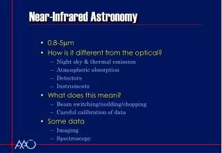
Near-Infrared Astronomy. 0.8-5 m How is it different from the optical? Night sky & thermal emission Atmospheric absorption Detectors Instruments What does this mean? Beam switching/nodding/chopping Careful calibration of data Some data Imaging Spectroscopy. >7.5 magnitudes!.

Near-Infrared Astronomy
E N D
Presentation Transcript
Near-Infrared Astronomy • 0.8-5m • How is it different from the optical? • Night sky & thermal emission • Atmospheric absorption • Detectors • Instruments • What does this mean? • Beam switching/nodding/chopping • Careful calibration of data • Some data • Imaging • Spectroscopy
>7.5 magnitudes! Far-IR Optical Near-IR H,NII,SII J,H,K Why?
Near-Infrared Sky • As wavelengths lengthen the sky gets brighter • Combined effects of • Moon/zodiacal (ie scattered solar spectrum) • OH airglow (forest of lines from 0.8mup) • Thermal emission (from sky dominates 2.4 mup) • The sky also absorbs a lot more light. • H20 absorption bands block regions from 0.8mup • The “gaps” between these bands define the “windows” or “bands” of IR astronomy. • Z,J,H,K,L,M,…. • Your instrument contributes • Without a cryogenic pupil stop, you get to “see” the thermal emission from your telescope, dome, and instrument.
The sky “brightness” of IR bands V(dark) 0.5 21.5 V(bright) 0.5 18.5 I (dark) 0.8 19.3 I (bright) 0.8 18.2
Bright Sky Thermal Dark Sky The near near-IR & the Moon
J Ks J Ks L M L M z’ H z’ H
When the Moon is not irrelevant in the IR • At high resolution - 3000 - we will see continuum sky “between” the OH lines. • Spectroscopy in near-IR will become a dark time observation
The sky is bright and highly variable. • If the sky was only bright, it would add to our S/N, but observing would be no different to the optical. • OH in z,J,H,Kshort bands. Thermal in Klong,L,M bands. • 2MASS prototype camera • H-band filter • 120”/pix, 256x256 pix • 30 frames over 45 minutes • Camera fixed • Moon & stars track across field • OH night-sky emission is very variable!
The sky is bright and highly variable. • In imaging and spectroscopy you need to “measure” the sky regularly, so you can subtract it • every few minute (imaging) to every 10-15 minutes (spectroscopy) • In imaging you achieve this by ‘dithering’ every few minutes • Because the sky is so bright there is rarely a read-noise penalty (typically 10-15e per read) in doing this • In spectroscopy you achieve this by ‘nodding’ your target on the slit (or nodding to sky) every 5-15 minutes • In spectroscopy you have to trade off between read noise (~10e) and sky brightness, to ensure you don’t get read noise dominated.
MultiSlit Slit Cold Stop Grism Main-dewar Fore-dewar E4470 TELESCOPE BACK FOCUS FLOOR OF CAGE INCREASED 50 MM 1370 COLLIMATORLENS ASEMBLY FILTER WHEEL SLIT WHEEL 80 110 COLD STOP WHEEL GRISM WHEEL FIELD LENS WINDOW FIELD FLATTENER INCOMING RADIATION TELESCOPE CENTRE LINE STEPPER MOTOR DETECTOR TRANSLATOR DETECTOR UNSWIRF(Upgrade) CAMERALENS ASSEMBLY PUPIL IMAGER TWO STAGE CRYO COOLER CRYO COOLER GAS 22MAR99 REVISED ANGLO-AUSTRALIAN OBSERVATORY MOUNTING PLANE OF A&G BOX CHKD IRIS2 LAYOUT - F/2.2 CAMERA GRASEBY SPECAC OPTICS 3RD. ANGLE PROJ. 0 20 40 80 160 ASS`Y DRAWING No. IRIS2 PROJECT DRAWINGNo. A-2 D E4470 REV. MILLIMETRES
Cold Stops and Cryogenics • Infrared detectors need to be kept cold (like optical detectors) • To control their own dark current and thermal emission • They also need cold stops • To control the telescope’s thermal emission • They also need the instrument and optical components held cold • To control the instrument’s thermal emission • As a result they are expensive and difficult to build. • Elements must be kept small. Elements can’t be interchanged. Everything is more difficult.
Detectors • HgCdTe (0.8-2.5m) and InSb (1-5m). • Read by multiplexers rather than charge shifting. Each pixel is addressed in sequence. • Must be read faster than CCDs. • Typically an array (1Kx1K or 2Kx2K) needs to be read in ~1s • Compare with 2Kx4K CCDs read speeds of 60s • Read noise is higher • Typically 10e- per read, or 14e- per double correlated sample • Multiple reads can lower this to 4-5e- for some applications. • Compare with <2e- for CCDs • Dark current is higher • Typically 1 to 0.1 e/pix/s.
Detectors • HgCdTe arrays are sometimes subject to “residual images” • Heavily saturated pixels may retain high dark current for some time • Effect is less in late model (HAWAII) detectors. • Read-out amplifiers can glow • This sets a limit to the number of reads which can be used to beat down read-noise. • Usually have significant non-linearity. • Can be as much as 5% near full-well.
“Up the ramp” Sample Read 1…n Double Correlated Sample Fowler Sample Read2 Reset Read (n+1) - (2n) Read1 Flux Reset Read1-n Reset Flux Flux Time Time Time Detector Read Modes • Double-correlated sampling (Flux=Read2-Read1). • Multiple Read modes • Fowler (Mean of n reads at end - mean of n reads at end) • “Up the ramp” (Least squares fit to n reads) • Total reads usually limited < 60-100 by read-out glow.
Some Data … from ESO SOFI 1Kx1K HgCdTe • Dark - vertical cut
Some Data … from ESO SOFI 1Kx1K HgCdTe • Dark - read-out glow & bad pixels.
Some Data … from ESO SOFI 1Kx1K HgCdTe • A Flat field in J
Some Data … from ESO SOFI 1Kx1K HgCdTe • Raw Data in J~500adu in sky10adu/e- • Quick-look attelescope ismost easily done by pair-wise subtraction
Some Data … from ESO SOFI 1Kx1K HgCdTe • HK R~1000 spectra Blue OH sky emission lines Thermal at red end of K Red
Some Data … from ESO SOFI 1Kx1K HgCdTe • HK R~1000 spectravertical cut
Some Data … from ESO SOFI 1Kx1K HgCdTe • HK R~1000 spectrahorizontal cut
Some Data … from ESO SOFI 1Kx1K HgCdTe • HK R~1000 spectrapair-wise subtraction
Planning your observations • Sky brightness and target brightness. • You have to be very aware of how bright your sky will be, how bright your target will be. Keep sky below half-full-well (or lower if non-linearity is significant). Keep target below full-well! • Read-noise and read-mode. • Make sure you are sky limited. You can make as many reads as you like, once you are sky limited. • Dark currents • Be aware of the dark current and associated noise. • Dead-times. • Be very aware of time to nod & settle telescope, time for a single, time for a detector read, and other overheads. These can be much more significant than in the optical.
Beam-switching Thought Experiments • Should be done as often as possible, without adding a read-noise or dead-time penalty. • Imaging in DCS, 14e- read noise, 0.5e-/s/pix dark current. 100000e- full well. Array read time 1.5s. Time to nod 10s. • J : Sky=3000e- in 10s. So sky noise=54e- in 10s. There is no read noise penalty in many reads. Dither ~ 120s to keep dead time down. • K : Sky=50000e- in 10s. Similar situation. Dither ~ 120s. • Spectroscopy in Fowler mode. 7e- read noise for 50 reads. So we must stay on target for at LEAST 75s. After 300s, dark current=150e/pix, dark noise=12e- so we are dark limited. • J : Sky in lines is 3000e- in 300s, but sky in gaps is 300e-, so we are just sky limited and can nod every 5 minutes. • K : Sky will be brighter than J. We can certainly nod every 5 minutes or faster, but should look at the bright thermal end to ensure we don’t hit full well.
Calibrations If you cheat on your calibrations, you will get all the trouble you deserve. • Flat fields • usually best constructed from dome, but taken in pairs with lamps on, and lamps off, to remove thermal effects of dome and instrument. • Darks/bias • usually best acquired for every exposure time and read-mode you use. You will also use these (and the flats) to determine which pixels are bad. • Arcs (ie wavelength calibration for spectra) • straightforward, but beware not to use bright arc lines on detectors with residual images. Arcs may be best taken at end of night. OH sky lines may provide all the calibration you need.
Calibrations • Atmospheric transmission (spectra) • usually almost featureless F and G star spectra. The combination will allow you to remove features from the star spectra. Everything else is due to the atmosphere. Take these frequently and close to your target on the sky - especially if you want to trust data at the edges of the atmospheric bands. • Photometric standards (imaging) • are self explanatory. However, you may want to take at least one rastered in a dense grid across your field of view, if your instrument has light concentration problems (most IR cameras do).
Data processing • Dark/bias subtraction : obvious. • Flat fielding • Use pixels which won’t flat-field/dark subtract to create a bad-pixel mask. IRAF will allegedly handle bad pixel masks now. Figaro and many Starlink packages certainly do. • Sky subtraction • Imaging : usually median (or median with sigma clipping, or average with sigma clipping) 5-7 normalized images taken near your target in time and on the sky. Then re-normalize this “sky” to your frame and subtract. • Spectroscopy : can do the above, but more usually simply subtract other frame from an object sky pair AB BA (ie A is sky for B) or the average of the spanning pair in an ABAB sequence.
Data Processing • If you are going to linearity correct your data you should do this after dark subtraction, but before flat fielding. • Once you have sky subtracted your data, • Imaging : you can use your favourite combination algorithm, or photometer all images separately. • Combination has the advantage you can ‘fill in’ bad pixels in a dithered data set. However, it can be a lot of work, and may actually give worse photometry than processing all data as separate images. • Spectroscopy: by this point your data should look much like optical data and further steps are pretty much the same.
Conclusions • Short of 2.3m consider the near-IR an extension of the optical. • Night sky emission makes life harder, but only slightly harder than the 0.8-1.0 m optical range. • Detectors are smaller and need to be more carefully processed • But this will change over your careers. • 2.3 m - 5 m is really “thermal” IR and quite different. • Backgrounds are high and variable. H2O absorption is strong and variable. Really only suited to high, dry sites like Chile & Mauna Kea.