Chapter 2: Simple Comparative Experiments (SCE)
Chapter 2: Simple Comparative Experiments (SCE). Simple comparative experiments: experiments that compare two conditions (treatments) The hypothesis testing framework The two-sample t -test Checking assumptions, validity. Portland Cement Formulation (page 23).

Chapter 2: Simple Comparative Experiments (SCE)
E N D
Presentation Transcript
Chapter 2: Simple Comparative Experiments (SCE) • Simple comparative experiments: experiments that compare two conditions (treatments) • The hypothesis testing framework • The two-sample t-test • Checking assumptions, validity
Portland Cement Formulation (page 23) • Average tension bond sterngths (ABS) differ by what seems nontrivial amount. • Not obvois that this difference is large enough imply that the two formulations really are diff. • Diff may be due to sampling fluctuation and the two formulations are really identical. • Possibly another two samples would give opposite results with strength of MM exceeding that of UM. • Hypothesis testing can be used to assist in comparing these formulations. • Hypothesis testing allows the comparison to be made on objective terms, with knowledge of risks associated with searching the wrong conclusion
Graphical View of the DataDot Diagram, Fig. 2-1, pp. 24 • Response variable is a random variable • Random variable: • Discrete • continuous
Box Plots, Fig. 2-3, pp. 26 • Displays min, max, lower and upper quartile, and the median • Histogram
Probability Distributions • Probability structure of a Random variable, y, is described by its probability distribution. • y is discrete: p(y) is the probability function of y (F2-4a) • y is continuous: f(y) is the probability density function of y (F2-4b)
Probability DistributionsProperties of probability distributions • y-discrete: • y-continuous:
Probability Distributionsmean, variance, and expected values
Probability DistributionsBasic Properties • E(c) = c • E(y) = m • E(cy) = c E(y) = c m • V(c) = 0 • V(y) = s2 • V(cy) = c2 V(y) = c2s2
Probability DistributionsBasic Properties • E(y1+y2) = E(y1)+E(y2) = m1+m2 • Cov(y1,y2) = E[(y1-m1)(y2-m2)] • Covariance: measure of the linear association between y1 and y2. • E(y1.y2) = E(y1).E(y2) = m1.m2 (y1 and y2 are indep)
Sampling and Sampling Distributions • The objective of statistical inference is to draw conclusions about a population using a sample from that population. • Random Sampling: each of N!/(N-n)!n! samples has an equal probability of being chosen. • Statistic: any function of observations in a sample that does not contain unknown parameters. • Sample mean and sample variance are both statistics.
Properties of sample mean and variance • Sample mean is a point estimator of population mean m • Sample variance is a point estimator of population variance s2 • The point estimator should be unbiased. Long run average should be the parameter that is being estimated. • An unbiased estimator should have min variance. Min variance point estimator has a variance that is smaller than the variance of any other estimator of that parameter.
Degrees of freedom • (n-1) in the previous eq is called the NDOF of the sum of squares. • NDOF of a sum of squares is equal to the no. of indep elements in the sum of squares • Because , only (n-1) of the n elements are indep, implying that SS has (n-1) DOF
The normal and other sampling distributions • Normal Distribution • y is distributed normally with mean m and variance s2 • Standard normal distribution: m=0 and s2=1
Central Limit Theorem • If y1, y2, …, yn is a sequence of n independent and identically distributed random variables with E(yi) = m and V(yi) = s2 (both finite) and x = y1+y2+…+yn, then has an approximate N(0,1) distribution. • This implies that the distribution of the sample averages follows a normal distribution with • This approximation require a relatively large sample size (n≥30)
Chi-Square or c2 distribution • If z1, z2, …, zn are normally and independently distributed random variables with mean 0 and variance 1 NID(0,1), then the random variable follows the chi-square distribution with k DOF.
Chi-Square or c2 distribution • The distribution is asymmetric (skewed) m = k s2= 2k • Appendix III
Chi-Square or c2 distribution • y1, y2, …, yn is a random sample from N(m,s), then • SS/s2 is distributed as chi-square with n-1 DOF
Chi-Square or c2 distribution • If the observations in the sample are NID(m,s), then thedistribution of S2is and, ,,, • Thus, the sampling distribution of the sample variance is a constant times the chi-square distribution if the population is normally distributed
Chi-Square or c2 distribution • Example: The Acme Battery Company has developed a new cell phone battery. On average, the battery lasts 60 minutes on a single charge. The standard deviation is 4.14 minutes. • Suppose the manufacturing department runs a quality control test. They randomly select 7 batteries. The standard deviation of the selected batteries is 6 minutes. What would be the chi-square statistic represented by this test? • If another sample of 7 battery was selected, what is the probability that the sample standard deviation is greater than 6? DOX 6E Montgomery
Chi-Square or c2 distribution Solution • a) We know the following: • The standard deviation of the population is 4.14 minutes. • The standard deviation of the sample is 6 minutes. • The number of sample observations is 7. • To compute the chi-square statistic, we plug these data in the chi-square equation, as shown below. • c2 = [ ( n - 1 ) * s2 ] / σ2c2 = [ ( 7 - 1 ) * 62 ] / 4.142 = 12.6 DOX 6E Montgomery
Chi-Square or c2 distribution • b) To find the probability of having a sample standard deviation S > 6, we refer to the Chi-square distribution tables, we find the value of a corresponding to chi-square = 12.6 and 6 degrees of freedom. • This will give a = 0.05 which is the probability of having S > 6 DOX 6E Montgomery
t distribution with k DOF • If z and are indpendent normal and chi-square random variables, the random variable • Follow t distribution with k DOF as follows:
t distribution with k DOF m = 0 and s2 = k/(k-2) for k>2 • If k=infinity, t becomes standard normal • If y1, y2, …, yn is a random sample from N(m,s), then is distributed as t with n-1 DOF
t distribution - example Example: • Acme Corporation manufactures light bulbs. The CEO claims that an average Acme light bulb lasts 300 days. A researcher randomly selects 15 bulbs for testing. The sampled bulbs last an average of 290 days, with a standard deviation of 56 days. If the CEO's claim were true, what is the probability that 15 randomly selected bulbs would have an average life of no more than 290 days? DOX 6E Montgomery
t distribution – Example Solution To find P(x-bar<290), • The first thing we need to do is compute the t score, based on the following equation: • t = [ x - μ ] / [ s / sqrt( n ) ] t = ( 290 - 300 ) / [ 56 / sqrt( 15) ] = - 0.692 • P(t<-0.692) is equivalent to P(t>0.692) DOX 6E Montgomery
t distribution – Example • From the t-distribution tables, we have a = 25% which correspond to the probability of having the sample average less than 290 DOX 6E Montgomery
F distribution • If and are two independent chi-square random variables with u and v DOF, then the ratio • Follows the F dist with u numerator DOF and v denominator DOF
F distribution • Two independent normal populations with common variance s2. If y11, y12, …, y1n1 is a random sample of n1 observations from 1st population and y21, y22, …, y2n2 is a random sample of n2 observations from 2nd population, then
The Hypothesis Testing Framework • Statistical hypothesis testing is a useful framework for many experimental situations • We will use a procedure known as the two-sample t-test
The Hypothesis Testing Framework • Sampling from a normal distribution • Statistical hypotheses:
Summary Statistics (pg. 36) Formulation 2 “Original recipe” Formulation 1 “New recipe”
How the Two-Sample t-Test Works: • Values of t0 that are near zero are consistent with the null hypothesis • Values of t0 that are very different from zero are consistent with the alternative hypothesis • t0 is a “distance” measure-how far apart the averages are expressed in standard deviation units • Notice the interpretation of t0 as a signal-to-noiseratio
The Two-Sample (Pooled) t-Test t0 = -2.20 • So far, we haven’t really done any “statistics” • We need an objective basis for deciding how large the test statistic t0 really is.
The Two-Sample (Pooled) t-Test t0 = -2.20 • A value of t0 between –2.101 and 2.101 is consistent with equality of means • It is possible for the means to be equal and t0 to exceed either 2.101 or –2.101, but it would be a “rareevent” … leads to the conclusion that the means are different • Could also use the P-value approach
Use of P-value in Hypothesis testing • P-value: smallest level of significance that would lead to rejection of the null hypothesis Ho • It is customary to call the test statistic significant when Ho is rejected. Therefore, the P-value is the smallest level a at which the data are significant.
Checking Assumptions – The Normal Probability Plot • Assumptions • Equal variance • Normality • Procedure: • Rank the observations in the sample in an ascending order. • Plot ordered observations vs. observed cumulative frequency (j-0.5)/n • If the plotted points deviate significantly from straight line, the hypothesized model in not appropriate.
Checking Assumptions – The Normal Probability Plot • The mean is estimated as the 50th percentile on the probability plot. • The standard deviation is estimated as the differnce between the 84th and 50th percentiles. • The assumption of equal population variances is simply verified by comparing the slopes of the two straight lines in F2-11.
Importance of the t-Test • Provides an objective framework for simple comparative experiments • Could be used to test all relevant hypotheses in a two-level factorial design.
Confidence Intervals (See pg. 43) • Hypothesis testing gives an objective statement concerning the difference in means, but it doesn’t specify “how different” they are • Generalform of a confidence interval • The 100(1- α)% confidenceinterval on the difference in two means:
Hypothesis testing • The test statitic becomes • This statistic is not distributed exactly as t. • The distribution of to is well approximated by t if we use as the DOF
Hypothesis testing • The test statitic becomes • If both populations are normal, or if the sample sizes are large enough, the distribution of zo is N(0,1) if the null hypothesis is true. Thus, the critical region would be found using the normal distribution rather than the t. • We would reject Ho, if where za/2 is the upper a/2 percentage point of the standard normal distribution
Hypothesis testing • The 100(1-a) percent confidence interval: