Download
1 / 27
270 likes | 497 Vues
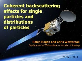
Coherent backscattering effects for single particles and distributions of particles . Robin Hogan and Chris Westbrook Deptartment of Meteorology, University of Reading. 25 March 2014. Overview. Motivation

E N D
Coherent backscattering effects for single particles anddistributionsof particles Robin Hogan and Chris Westbrook Deptartment of Meteorology, University of Reading 25 March 2014
Overview • Motivation • We need to be able to model the backscattered signal from clouds in order to interpret radar and lidar observations (particularly from space) in terms of cloud properties • Coherent backscattering effects for single particles • Radar scattering by ice aggregates and snowflakes • The Rayleigh-Gans approximation • A new equation for the backscatter of an ensemble of ice aggregates: the Self-Similar Rayleigh-Gans approximation • Coherent backscattering effects for distributions of particles • Coherent backscatter enhancement (CBE) for solar illumination • The multiple scattering problem for radar and lidar • How important is CBE for radar and lidar? • A prediction • Coherent backscatter enhancement occurs for individual particles so ray tracing could underestimate backscattering by a factor of two
The principle unifying this talk Single particle Distribution of particles Backscattered amplitude is found by summing the returned rays coherently
Radar observations of tropical cirrus • Two airborne radars: 3 mm (94 GHz) and 3 cm (10 GHz) • Most ice particles scatter in Rayleigh regime only for 3-cm radar • How can we interpret deviations from Rayleigh scattering in terms of particle size? 3-mm wavelength scattered 100 times less 3-mm wavelength scattered 10 times less 3-mm wavelength in Rayleigh regime Hogan et al. (2012)
Two problems • Snowflakes have complicated shapes • Methods to compute their scattering properties are slow Is the best we can do to (somehow)generate a large ensemble of 3D snowflake shapes and compute their scattering by brute force? Potentially not: • Snowflakes have fractal structure that can be described statistically • The Rayleigh-Gans approximation is applicable Images from Tim Garrett, University of Utah
The Rayleigh-Gansapproximation Aggregate from Westbrook et al. (2004) model Backscatter depends only on A(s) function and dielectric constant e (or refractive index m = e1/2) Distance s Area A(s)
The Rayleigh-Gans approximation Mean structure, k = kurtosis parameter Fluctuations from the mean • Backscatter cross-section is proportional to the power in the Fourier component of A(s) at the scale of half the wavelength • Can we parameterize A(s) and its variation? • where and V is the volume of ice in the particle
Aggregate mean structure • Hydrodynamic forces cause ice particles to fall horizontally, so we need separate analysis for horizontally and vertically viewing radar • Mean structure of 50 simulated aggregates is very well captured by the two-cosine model with kurtosis parameters of • k = –0.11 for horizontal structure • k = 0.19 for vertical structure
Aggregate self-similar structure Aggregates of bullet rosettes Aggregate structure: -5/3 Solid ice: -4 Power spectrum of fluctuations obeys a -5/3 power law • Why the Kolmogorov value when no turbulence involved? Coincidence? • Aggregates of columns and plates show the same slope (Physical scale: D/j )
New equation • Assumptions: • Power-law: • Fluctuations at different scales are uncorrelated: • Sins and cosine terms at the same scale are uncorrelated: • Leads to the Self-Similar Rayleigh-Gans approximation for backscatter coefficient: • where Hogan and Westbrook (2014, in revision)
Radar scattering by ice 1 mm ice 1 cm snow • Internal structures on scale of wavelength lead to significantly higher higher backscatter than “soft spheroids” (proposed by Hogan et al. 2012 and others) Realistic snowflakes “Soft spheroid”
Field et al. (2005) size distributions at 0°C Circles indicate D0 of 7 mm reported from aircraft (Heymsfield et al. 2008) Lawson et al. (1998) reported D0=37 mm: 17 dB difference Impact of scattering model 4.5 dB Factor of 5 error Ice water content (g m-3) Radar reflectivity factor (dBZ)
Ice aggregates Ice spheres Impact of ice shape on retrievals • Spheres can lead to overestimate of water content and extinction of factor of 3 • All 94-GHz radar retrievals affected in same way
Why are Saturn’s rings brighter when the sun is in opposition? • Shadow hiding in the icy rocks that compose the rings (r >> l)? • Coherent backscatter enhancement (r<= l)? • Multiply scattered light paths normally add incoherently • But for every path L1P1P2…PnL2 there is an equivalent reverse path L1PnPn-1…P1L2 whose length differs by only • Where Dx is the lateral distance between the first and last particles in the scattering chain (P1Pn in this example) • These paths will add coherently if Dp << l • Reflected power twice what it would be for incoherent averaging Dx L2 L1
Observed enhancement Define coherent backscatter enhancement (0 = none, 1 = doubled reflection) for single pair of multiply scattered paths as Observed enhancement found by integrating over distribution of Dx: If this distribution is Gaussian with width s, then integral evaluates as: where But remember that there is no enhancement for single scattering, so this effect is only observed if multiple scattering is significant
Laboratory measurements • Measurements by Wolf et al. (1985)
Dependence on source • Confined source (radar or lidar) • Distance Dx determined by field-of-view of transmitter and receiver: transmitted light returning outside the FOV is not detected • Lower Dx implies higher enhancement, but overall multiple scattering return is lower • Very little literature • Extended source (e.g. sun) • Distance Dx determined by mean free path of light in the cloud of particles • Most of the literature concerns this case Cloud of scatterers Dx
Examples of multiple scattering Stratocumulus Surface echo Apparent echo from below the surface Intense thunderstorm • LITE lidar (l<r, footprint~1 km) • CloudSat radar (l>r)
Fast multiple scattering modelHogan and Battaglia (JAS 2008) Uses the time-dependent two-streamapproximation Agrees with Monte Carlo but ~107 times faster (~3 ms) Used in CloudSat operational retrieval algorithms CloudSat-like example CALIPSO-like example
Moving platform: satellite radar or lidar • Consider CloudSat & Calipso satellites at altitude of 700 km and speed of 7 km s-1: • Distance travelled between time of reception and transmission is l = 33 m • So q = 47 mrad • Assuming most multiply scattered light escapes field-of-view, s determined by receiver footprint on the cloud • CloudSat: s = 450 m, l = 3 mm so • CBE = 10-9 • Calipso: s = 100 m, l = 0.5 mm so • CBE = 0 • Effect can be safely ignored for satellites
Stationary platform: ground-based • And even for a monostatic radar, can’t radiation be received from a different part of the antenna to where it was transmitted? • q = 0 so automatically we have CBE = 1 and the multiply scattered return is doubled? • But most lidars are bistatic!
Stationary lidar • Treat laser as infinitesimal point and integrate over all possible transmit-receive distances l: • CBE is close to zero! Transmit-receive distance l Telescope Laser Centreline offset l0 Telescope radius r0
Stationary radar • Again need to integrate over all possible transmit-receive distances • Complication is that beam pattern is diffraction limited: field-of-view (and hence s) is dependent on transmit-receive distance… • Stationary radar should have fixed value of CBE, probably around 0.5, but theory needs to be developed Transmit-receive distance l
_______ ___________ ___________ ___ _________ Coherent backscatter enhancement for particles? • Predictions for light scattering by particles r>>l: • Coherent effects should double the backscatter due to light rays involving more than 1 reflection • The angular width of the enhancement is of order where s is the RMS distance between entering and exiting light rays. • For 100 mm particles and l=0.5 mm, q0 is 0.05 degrees • Ray tracing codes are unlikely to capture this effect, but explicit solutions of Maxwell’s equations will (Mie, DDA)
_______ __________ ________ Standard scattering patterns Hogan (2008) Liquid spheres (Mie theory) • Width of backscatter peak is dependent on particle size • Is this peak underestimated by ray tracing? • Ice particle phase functions • Ping Yang’s functions show size-independent enhancement of a factor of ~8 • Anthony Baran’s functions are flat at backscatter • Neither seems right; do we need to model CBE?
Summary • A new equation has been proposed for backscatter cross-section of ice aggregates observed by radar • Much higher 94-GHz backscatter for snow than “soft spheroids” • Aggregate structure exhibits a power law with a slope of -5/3: why? • Coherent backscatter enhancement (CBE) has been estimated for spaceborne and ground-based radar and lidar: • From space it can be neglected because of the distance travelled between transmission and receiption • From the ground, the finite size of a lidar laser/telescope assembly also makes CBE negligible • CBE can be significant for a ground based radar, and the exact value should be instrument/wavelength independent for monostatic radars, but value has not yet been rigorously calculated • Coherent backscatter enhancement should apply to individual particles • Do current ray tracing algorithms underestimate backscattering by a factor of two because of this?