Download
1 / 35
370 likes | 616 Vues
KINEMATICS OF PARTICLES. Kinematics of Particles. This lecture introduces Newtonian (or classical) Mechanics. It concentrates on a body that can be considered as a single particle. This simply means that the size and shape of the body will not affect the solution of the problem.

E N D
KINEMATICS OF PARTICLES
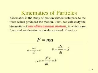
Kinematics of Particles • This lecture introduces Newtonian (or classical) Mechanics. It concentrates on a body that can be considered as a single particle. This simply means that the size and shape of the body will not affect the solution of the problem. • The lecture discusses the motion of a particle in 3-D space • After this lecture, the student should understand the following concepts: • Newtonian Mechanics in terms of statics and dynamics • Understand the logical division of Dynamics into kinematics and kinetics • Solve problems in kinematics of particles
Rigid Bodies Deformable Bodies Fluids Statics: concerns the equilibrium of bodies under the action of forces Dynamics: concerns the motion of bodies Kinematics: concerns the geometry of motion independent of the forces that produce the motion Kinetics: concerns the relationship between motion, mass, and forces What is Mechanics? • Science that describes and predicts the conditions of rest or motion of bodies under the action of forces Mechanics
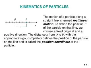
Review of Basic Concepts • Space = geometric region in which events take place. For general engineering applications, most machines will operate and move in 3-D space. Other examples: • Motion in a straight line, e.g. along the the x-axis 1-D space • Motion in a plane, e.g. along the x-y plane 2-D space • The concept of space is associated with position and orientation. Any point in 3-D space can be defined by 3 coordinates: x, y, and z measured from a certain reference point. The orientation of a machine can be defined by 3 rotational angles , , and about : x, y, and z axes respectively. These coordinates refer to a “System for Referencing” the position and orientation. • Both position/oritnation and time have to be used to define an event in space • Mass is used to characterize the bodies in space
Newtonian Mechanics Assumptions • There exists a primary inertial frame of reference fixed in space • Measurements made w.r.t. this reference is absolute • Time, space and mass are absolute • Interaction between particles is instantaneous The assumptions are invalid if velocities involved are of the same order as the speed of light! For most engineering problems of machines on earth’s surface, the assumptions are valid. For rockets and space-flight trajectories, using the assumptions may result in large errors
Inertial Frame An inertial frame is one in which the principles of Galileo and Newton holds true, i.e. a body will remain at rest or continue with uniform velocity in a straight line unless it is compelled to change its state of rest or uniform rectilinear motion by some external influence. A frame of reference is NOT inertial if a body not acted upon by outside influences accelerates on its own accord. All frames moving with rectilinear velocity with respect to the inertial frame are also inertial frames.
Z-axis vt* X-axis Y-axis Galileo’s relative principle Frame {a} = (X,Y,Z,t) is fixed and frame {b} = (e1,e2,e3,t1) is moving at constant velocity (v) in the direction of the positive X-axis, i.e. At t=t1=0, the two frames are together. At t1= t=t*, frame {b} has moved away from frame {a}
Z-axis vt* X-axis Y-axis At t1= t1=t* Galileo’s relative principle Let the position of particle “P” referenced w.r.t frame {a} be (x, y, z) and w.r.t. frame {b} be (x’, y’, z’) P
Velocity of P in frame {b} Velocity of frame {b} relative to {a} Velocity of P in frame {a} Galileo’s relative principle
Acceleration unchanged Galileo’s relative principle: A body un-accelerated in the frame {a} is also un-accelerated in all frames moving with constant velocity w.r.t. frame {a} Galileo’s relative principle
Z-axis :are the unit vectors for X,Y and Z-axis respectively Z X Y X-axis Y-axis Right-handed system We will use the right handed system of Cartesian coordinates to define a frame of reference: O
Perpendicular to each other Unit vectors X Note the cyclic cycle of the right hand system Y Z Right-handed system Note that the unit vectors for the right handed Cartesian reference frame are orthonormal basis vectors, i.e. The cross and dot products are defined as follow:
Z-axis The vector (e.g. ) defines the position of particle “A” w.r.t. frame {a}. In the e.g., the particle is 1 unit along the positive x-axis, 2 units along the positive y-axis and 3 units along the positive z-axis Particle “A” X-axis Y-axis Position With a frame of reference established, we can define the position of a particle “A” w.r.t. the frame at any instance of time using vectors: O This is called the parametric description of the position vector Frame {a}=(X,Y,Z)
Z-axis The position of particle “A” along the path at any instance of time can be represented by Particle “A” at time t1 Particle “A” at time t2 E.g. : at time t=t1=1, the particle is at the point [1, 1, 1]T and at time t=t2=2, the particle is at the point [2, 4, 8]T X-axis Y-axis Path of particle “A” Path The changes in position of a particle “A” with time w.r.t. the frame of reference can be described by a path:
E.g. : At time t1=1, At time t2=2, Average Velocity Given Let and denote the position at time t1 and t2 respectively. The AVERAGE velocity of a particle “A” between time t1 and t2 w.r.t. the frame of reference can be defined as: Average velocity between two points is defined as a vector w.r.t. the reference frame
E.g. : The velocity is At time t1=1, the instantaneous velocity is [1, 2, 3]T At time t2=2, the instantaneous velocity is [1, 4, 12]T Instantaneous velocity at any point is a vector defined w.r.t. the reference frame. It is tangential to the path at that point, i.e. along Instantaneous Velocity Given The instantaneous velocity of a particle “A” at any point along the path w.r.t. the frame of reference can be defined as:
Z-axis Direction of the instantaneous velocity at time t1 (tangential to the path) Changes with time Direction of the average velocity X-axis Y-axis Direction of instantaneous velocity at time t2 (tangential to the path) Average vs. Instantaneous Velocity Average and instantaneous velocity are not the same. Below shows the path of a particle between two position vectors at time t1 and t2:
t becomes smaller In this case, the average velocity will approaches the instantaneous velocity at t1: i.e. Notice that the direction of will be tangential to the curve in the limit as t0, i.e. the instantaneous velocity is tangential to the path. The tangential vector is called Average vs. Instantaneous Velocity Notice that if the time interval between t1 and t2 becomes smaller, i.e. t0, then
Example: The instantaneous velocity of a particle is The instantaneous speed of the particle has no direction : Speed and Velocity Speed and velocity are not the same! Velocity is a vector (it has both magnitude an direction). Speed “v” is a scalar. Speed only refers to the magnitude of the velocity, i.e.. Just as there are instantaneous and average velocities, there are also instantaneous and average speed.
E.g. : The acceleration is At time t1=1, the particle acceleration is [0, 2, 6]T At time t2=2, the particle velocity is [0, 2, 12]T Instantaneous Acceleration Given The instantaneous acceleration of a particle “A” at any point along the path w.r.t. the frame of reference can be defined as: Instantaneous acceleration at any point is a vector defined w.r.t. the reference frame.
Z-axis Particle “A” at time t1 Particle “A” at time t2 E.g. Find the distance traveled between t1=0 and t2=1 sec. X-axis Y-axis “s” is the distance traveled Arc Length The total distance traveled by the particle “A” between time t1 and t2 is described by the arc length “s”:
But the instantaneous speed is the magnitude of the instantaneous velocity, which is tangential along the path, i.e. along the vector In this case, we can also define the instantaneous velocity as where Arc Length, Speed and Velocity The arc length is given as: The instantaneous speed is defined as: Therefore, it is obvious that instantaneous speed is:
Using the arc length “s”, we can defined the normal vector as where is called the curvature The binormal vector is defined as The three unit vectors are orthonormal basis vectors and form a right handed reference frame. Together, they are called the trihedron. Tangential, Normal and Binormal vectors Given we can defined the tangential vector
The radius of curvature is defined as Trihedron The trihedron can be determined as follow: The curvature can be found using The torsion is defined as
Trihedron Example Given find the trihedron at time t Solution:
Trihedron Example Story so far:
Z-axis Z-axis Note that: We let az az ax X-axis X-axis Y-axis Y-axis ay r Cylindrical Coordinates A position vector can be defined using a Cartesian reference frame as
r The magnitude of the velocity is Quick Review of circular motion A quick review of velocity in planar circular motion: consider a particle that moves in a circle with a fixed angular velocity The direction of the velocity is always tangential to the curve
define a new coordinate system called the cylindrical coordinates. If we look at “r” and in the x-y plane: Z-axis Y-axis r az X-axis X-axis Y-axis r Cylindrical Coordinates
Y-axis Y-axis v vr X-axis X-axis Cylindrical Coordinates Similarly, replacing r with vr and v where
Cylindrical Coordinates Summary:
A position vector can be defined using Cylindrical coordinates as Note that: Z-axis Z-axis We let az X-axis X-axis Y-axis Y-axis R r Spherical Coordinates
define a new coordinate system called the spherical coordinates. We know that: Z-axis Z-axis R R X-axis Y-axis r-axis r Spherical Coordinates If we look at “R” and in the ‘r-R’ plane:
Spherical Coordinates Similarly we can replace “R” with vR, v and v and repeat the analysis to get:
Summary • This lecture concentrates on a body that can be considered as a particle and discusses the motion of a particle in 3-D space • The following concepts were covered: • Newtonian Mechanics in terms of statics and dynamics • The logical division of Dynamics into kinematics and kinetics • Problems in kinematics of particles • In the treatment of a body as a particle, the shape and size of the body is not considered.