Download

1 / 18
210 likes | 596 Vues
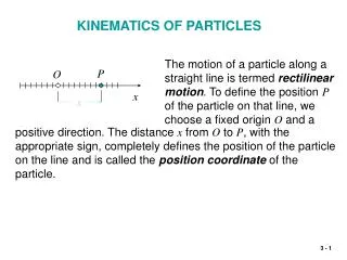
KINEMATICS OF PARTICLES RELATIVE MOTION WITH RESPECT TO TRANSLATING AXES.

E N D
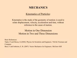
KINEMATICS OF PARTICLES RELATIVE MOTION WITH RESPECT TO TRANSLATING AXES
In the previous articles, we have described particle motion using coordinates with respect to fixed reference axes. The displacements, velocities and accelerations so determined are termed “absolute”. It is not always possible or convenient, however, to use a fixed set of axes to describe or to measure motion. In addition, there are many engineering problems for which the analysis of motion is simplified by using measurements made with respect to a moving reference system. These measurements, when combined with the absolute motion of the moving coordinate system, enable us to determine the absolute motion in question. This approach is called the “ relative motion analysis”.
The motion of the moving coordinate system is specified with respect to a fixed coordinate system. In Newtonian mechanics, this fixed system is the primary inertial system, which is assumed to have no motion in space. For engineering purposes, the fixed system may be taken as any system whose absolute motion s negligible for the problem at hand.
For most earthbound engineering problems, it is sufficiently precise to take for the fixed reference system a set of axes attached to the earth, in which case we neglect the motion of the earth. For the motion of satellites around the earth, a nonrotating coordinate system is chosen with its origin on the axis of rotation of the earth. For interplanetary travel, a nonrotating coordinate system fixed to the sunwould be used. Thus, the choice of the fixed system depends on the type of problem involved.
In this article, we will confine our attention to moving reference systems which translate but do not rotate. Motion measured in rotating systems will be discussed in rigid body kinematics, where this approach finds special but important application. We will also confine our attention here to relative motion analysis for plane motion.
Now let’s consider two particles A and B which may have separate curvilinear motions in a given plane or in parallel planes; the positions of the particles at any time with respect to fixed OXY reference system are defined by and . Let’s arbitrarily attach the origin of a set of translating (nonrotating) axes to particle B and observe the motion of A from our moving position on B. Y y A x B X O
The position vector of A as measured relative to the frame x-y is , where the subscript notation “A/B” means “A relative to B” or “A with respect to B”. The unit vectors along the x and y axes are and , and x and y are the coordinates of A measured in the x -y frame. The absolute position of B is defined by the vector measured from the origin of the fixed axes X -Y. Y y A x B X O
The position of A is, therefore, determined by the vector Y y A x B X O
We now differentiate this vector equation once with respect to time to obtain velocities and twice to obtain accelerations. Here, the velocity which we observe A to have from our position at B attached to the moving axes x-y is . This term is the velocity of A with respect to B.
Acceleration is obtained as Here, the acceleration which we observe A to have from our nonrotating position on B is . This term is the acceleration of A with respect to B. We note that the unit vectors and have zero derivatives because their directions as well as their magnitudes remain unchanged.
The velocity and acceleration equations state that the absolute velocity (or acceleration) equals the absolute velocity (or acceleration) of B plus, vectorially, the velocity (or acceleration) of A relative to B. The relative term is the velocity (or acceleration) measurement which an observer attached to the moving coordinate system x-y would make. We can express the relative motion terms in whatever coordinate system is convenient – rectangular, normal and tangential or polar, and use their relevant expressions.
y Y A x B X O The selection of the moving point B for attachment of the reference coordinate system is arbitrary. Point A could have been used just as well for the attachment of the moving system, in which case the three corresponding relative-motion equations for position, velocity and acceleration are
y Y A x B X O It is seen, therefore, that In relative-motion analysis, it is important to realize that the acceleration of a particle as observed in a translating system x-y is the same as that observed in a fixed system X-Y if the moving system has a constant velocity.
PROBLEMS 1. The car A has a forward speed of 18 km/h and is accelerating at 3 m/s2. Determine the velocity and acceleration of the car relative to observer B, who rides in a nonrotating chair on the Ferris wheel. The angular rate = 3 rev/min of the Ferris wheel is constant.
PROBLEMS 2. Car A is travelling at the constant speed of 60 km/h as it rounds the circular curve of 300 m radius and at the instant represented is at the position q = 45°. Car B is travelling at the constant speed of 80 km/h and passes the center of the circle at this same instant. Car A is located with respect to car B by polar coordinates r and q with the pole moving with B. For this instant determine vA/B and the values of and as measured by an observer in car B.
PROBLEMS 3. Airplane A is flying horizontally with a constant speed of 200 km/h and is towing the glider B, which is gaining altitude. If the tow cable has a length r = 60 m and q is increasing at the constant rate of 5 degrees per second, determine the magnitudes of the velocity and acceleration of the glider for the instant when q = 15°.
PROBLEMS 4. After starting from the position marked with the “x”, a football receiver B runs the slant-in pattern shown, making a cur at P and thereafter running with a constant speed vB= 7 m/s in the direction shown. The quarterback releases the ball with a horizontal velocity of 30 m/s at the instant the receiver passes point P. Determine the angle a at which the quarterback must throw the ball, and the velocity of the ball relative to the receiver when the ball is caught. Neglect any vertical motion of the ball.
PROBLEMS 5. A batter hits the baseball A with an initial velocity of v0=30 m/s directly toward fielder B at an angle of 30° to the horizontal; the initial position of the ball is 0.9 m above ground level. Fielder B requires ¼ s to judge where the ball should be caught and begins moving to that position with constant speed. Because of great experience, fielder B chooses his running speed so that he arrives at the “catch position” simultaneously with the ball. The catch position is the field location at which the ball altitude is 2.1 m. Determine the velocity of the ball relative to the fielder at the instant the catch is made.