Chapter 20 Understanding Language
360 likes | 711 Vues
Chapter 20 Understanding Language. Chapter 20 Contents (1). Natural Language Processing Morphologic Analysis BNF Rewrite Rules Regular Languages Context Free Grammars Context Sensitive Grammars Recursively Enumerable Grammars Parsing Transition Networks Augmented Transition Networks.

Chapter 20 Understanding Language
E N D
Presentation Transcript
Chapter 20 Understanding Language
Chapter 20 Contents (1) • Natural Language Processing • Morphologic Analysis • BNF • Rewrite Rules • Regular Languages • Context Free Grammars • Context Sensitive Grammars • Recursively Enumerable Grammars • Parsing • Transition Networks • Augmented Transition Networks
Chapter 20 Contents (2) • Chart Parsing • Semantic Analysis • Ambiguity and Pragmatic Analysis • Machine Translation • Language Identification • Information Retrieval • Stemming • Precision and Recall
Natural Language Processing • Natural languages are human languages such as English and Chinese, as opposed to formal languages such as C++ and Prolog. • NLP enables computer systems to understand written or spoken utterances made in human languages.
Morphologic Analysis • The first analysis stage in a NLP system. • Morphology: the components that make up words. • Often these components have grammatical significance, such as “-es”, “-ed”, “-ing”. • Morphologic analysis can be useful in identifying which part of speech (noun, verb, etc.) a word is. • This is vital for syntactic analysis. • Identifying parts of speech can be done by having a list of standard endings (such as “-ly” – adverb). • This works well for regular verbs, but will not work for irregular verbs such as “go”.
BNF (1) • A grammar defines the syntactic rules for a language. • Backus-Naur Form (or Backus Normal Form) is used to write define a grammar in terms of: • Terminal symbols • Non-terminal symbols • The start symbol • Rewrite rules
BNF (2) • Terminal symbols: the symbols (or words) that are used in the language. In English, these are the letters of the Roman alphabet, for example. • Non-terminal symbols: symbols such as noun, verb that are used to define parts of the language. • The start symbol represents a complete sentence. • Rewrite rules define the structure of the grammar.
Rewrite Rules • For example: Sentence NounPhrase VerbPhrase • The rule states that the item on the left can be rewritten in the form on the right. • This rule says that one valid form for a sentence is a Noun Phrase followed by a Verb Phrase. • Two more complex examples: NounPhrase Noun | Article Noun | Adjective Noun | Article Adjective Noun VerbPhrase Verb | Verb NounPhrase | Adverb Verb NounPhrase
Regular Languages • The Simplest type of grammar from Chomsky’s hierarchy. • Regular languages can be described by Finite State Automata (FSAs) • A regular expression is a sentence defined by a regular language. • Regular languages are of interest to computer scientists, but are no use for NLP, as they cannot describe even simple formal languages, let alone human languages.
Conext Free Grammars • The rewrite rules we saw above define a context-free grammar. • They define what words can be used together, but do not take into account context. • They allow sentences that are not grammatically correct, such as: Chickens eats dog. • A context free grammar can have at most one terminal symbol on the right hand side of its rewrite rules.
Context Sensitive Grammars • A context sensitive grammar can have more than one terminal symbol on the RHS of its rewrite rules. • This allows the rules to specify context – such as case, gender and number. E.g.: A X B A Y B • This says that in the context of A and B, X can be rewritten as Y.
Recursively Enumerable Grammars • The most complex grammars in Chomsky’s hierarchy. • There are no rules to limit the rewrite rules of these grammars. • Also known as unrestricted grammars. • Not useful for NLP.
Parsing • Parsing involves determining thesyntactic structure of a sentence. • Parsing first tells us whether a sentence is valid or not. • A parsed sentence is usually represented as a parse tree. • The tree shown here is for the sentence “the black cat crossed the road”.
Transition Networks • Transition networks are FSAs used to represent grammars. • A transition network parser uses transition networks to parse. • In the following examples, S1 is the start state; the accepting state has a heavy border. • When a word matches an arc in a current state, the arc is followed to the new state. • If no match is found, a different transition network must be used.
Transition Networks – examples (2) • These transition networks represent rewrite rules with terminal symbols:
Augmented Transition Networks • ATNs are transition networks with the ability to apply conditions (such as tests for gender, number or case) to arcs. • Each arc has one or more procedures attached to it that checks conditions. • These procedures are also able to build up a parse tree while the network is applied to a sentence.
Inefficiency • Using transition networks to parse sentences such as the following can be inefficient – it will involve backtracking if the wrong interpretation is made: Have all the fish been fed? Have all the fish.
Chart Parsing (1) • Chart parsing avoids the backtracking problem. • At most, a chart parser will examine a sentence of n words in O(n3) time. • Chart parsing involves manipulating charts which consist of edges, vertices and words:
Chart Parsing (2) • The edge notation is as follows: [x, y, A B ● C] • This edge connects nodes x and y; It says that to create an A, we need a B and a C; The dot shows that we have already found a B, and need to find a C.
Chart Parsing (3) • To start with, a chart is as shown above. • The chart parser can add edges to the chart according to these rules: 1) If we have an edge [x, y, A B ● C], an edge can be added that supplies that C – i.e. the edge [x, y, C ● E], where E can be replaced by a C. 2) If we have [x, y, A B ● C D] and [y, z, C E ●] then we can form the edge: [x, z, A B C ● D]. 3) If we have an edge [x, y, A B ● C] and the word at y is of type C then we can add: [y, y+1, A B C ●].
Semantic Analysis • Aftering determining the syntactic structure of a sentence, we need to determine its meaning: semantics. • We can use semantic nets to represent the various components of a sentence, and their relationships. E.g.:
Ambiguity and Pragmatic Analysis • Unlike formal languages, human languages contain a lot of ambiguity. E.g.: • “General flies back to front” • “Fruit flies like a bat” • The above sentences are ambiguous, but we can disambiguate using world knowledge (fruit doesn’t fly). • NLP systems need to use a number of approaches to disambiguate sentences.
Ambiguity and Pragmatic Analysis • Unlike formal languages, human languages contain a lot of ambiguity. E.g.: • “General flies back to front” • “Fruit flies like a bat” • The above sentences are ambiguous, but we can disambiguate using world knowledge (fruit doesn’t fly). • NLP systems need to use a number of approaches to disambiguate sentences.
Syntactic Ambiguity • This is where a sentence has two (or more) correct ways to parse it:
Semantic Ambiguity • Where a sentence has more than one possible meaning. • Often as a result of syntactic ambiguity.
Referential Ambiguity • Occurs as a result of a use of anaphoric expressions: John gave the ball to the dog. It wagged its tail. • Was it John, the ball or the dog that wagged? • Of course, humans know the answer to this: an NLP system needs world knowledge to disambiguate.
Disambiguation • Probabilistic approach: • The word “bat” is usually used to refer to the sporting implement. • The word “bat”, when used in a scientific article, usually means the winged mammal. • Context is also useful: • “I went into the cave. It was full of bats.” • “I looked in the locker. It was full of bats.” • A good, relevant world model with knowledge about the universe of discourse is vital.
Machine Translation • One of the earliest goals of NLP. • Indeed – one of the early goals of AI. • Translating entire sentences from one human language to another is extremely difficult to automate. • Ambiguities in one language may not be ambiguous in another (e.g. “bat”). • Syntax and semantics are usually not enough – world knowledge is also needed. • Machine translation systems exist (e.g. Babelfish) but none have 100% accuracy.
Language Identification • Similar problem to machine translation – but much easier. • Particularly useful with Internet documents which usually have no indication of which language they are in. • Acquaintance algorithm uses n-grams. • An n-gram is a collection of n letters. • Statistics exist which correlate 3-grams with languages. • E.g. “ing”, “and”, “ent” and “the” occur very often in English but less frequently in other languages.
Information Retrieval • Matching queries to a corpus of documents (such as the Internet). • One approach uses Bayes’ theorem: • This assumes that the most important words in a query are the least common ones. • E.g. if “elephants in New York” is submitted as a query to the New York Times, the word “elephants” is the one that contains the most information. • Stop words are ignored – “the”, “and”, “if”, “not”, etc.
TF – IDF (1) • Term Frequency - Inverse Document Frequency. • Inverse Document Frequency for a word is: • |D| is the number of documents in the corpus. • DF (W) is the number of documents in the corpus that have the word W. • TF (W, D) is the number of times word W occurs in document D.
TF – IDF (2) • The TF-IDF value for a word and document is: TF-IDF (D, Wi) = TF(Wi, D) x IDF (Wi) • This is calculated as a vector for each document, using the words in the query. • This gives high priority to words that occur infrequently in the corpus, but frequently in a particular document. • Then the document whose TF-IDF vector has the greatest magnitude is the one that is considered to be most relevant to the query.
Stemming • Removing common suffices from words (such as “-ing”, “-ed”, “-es”). • Means that a query “swims” will match “swimming”, “swimmers”. • Porter’s algorithm is the one most commonly used. • Has been shown to give some improvement in the performance of Information Retrieval systems. • Not good when applied to names – e.g. “Ted Turner” might match “Ted turned”.
Precision and Recall • 100% precision means no false positives: • All returned documents are relevant. • 100% recall means no false negatives: • All relevant documents will be returned. • In practice, high precision means low recall and vice-versa. • The holy grail of IR is to have high precision and high recall.