Optimizing LDPC Codes for message-passing decoding.
Optimizing LDPC Codes for message-passing decoding. Jeremy Thorpe Ph.D. Candidacy 2/26/03. Overview. Research Projects Background to LDPC Codes Randomized Algorithms for designing LDPC Codes Open Questions and Discussion. Data Fusion for Collaborative Robotic Exploration.

Optimizing LDPC Codes for message-passing decoding.
E N D
Presentation Transcript
Optimizing LDPC Codes for message-passing decoding. Jeremy Thorpe Ph.D. Candidacy 2/26/03
Overview • Research Projects • Background to LDPC Codes • Randomized Algorithms for designing LDPC Codes • Open Questions and Discussion
Data Fusion for Collaborative Robotic Exploration • Developed a version of the Mastermind game as a model for autonomous inference. • Applied the Belief Propagation algorithm to solve this problem. • Showed that the algorithm had an interesting performance-complexity tradeoff. • Published in JPL's IPN Progress Reports.
Dual-Domain Soft-in Soft-out Decoding of Conv. Codes • Studied the feasibility of using the Dual SISO algorithm for high rate turbo-codes. • Showed that reduction in state-complexity was offset by increase in required numerical accuracy. • Report circulated internally at DSDD/HIPL S&S Architecture Center, Sony.
Short-Edge Graphs for Hardware LDPC Decoders. • Developed criteria to predict performance and implementational simplicity of graphs of Regular (3,6) LDPC codes. • Optimized criteria via randomized algorithm (Simulated Annealing). • Achieved codes of reduced complexity and superior performance to random codes. • Published in ISIT 2002 proceedings.
Evalutation of Probabilistic Inference Algorithms • Characterize the performance of probabilistic algorithms based on observable data • Axiomatic definition of "optimal characterization" • Existence, non-existence, and uniqueness proofs for various axiom sets • Unpublished
Optimized Coarse Quantizers for Message-Passing Decoding • Mapped 'additive' domains for variable and check node operations • Defined quantized message passing rule in these domains • Optimized quantizers for 1-bit to 4-bit messages • Submitted to ISIT 2003
Graph Optimization using Randomized Algorithms • Introduce Proto-graph framework • Use approximate density evolution to predict performance of particular graphs • Use randomized algorithms to optimize graphs (Extends short-edge work) • Achieves new asymptotic performance-complexity mark
The Channel Coding Strategy • Encoder chooses the mth codeword in codebook C and transmits it across the channel • Decoder observes the channel output y and generates m’ based on the knowledge of the codebook C and the channel statistics. Encoder Channel Decoder
Linear Codes • A linear code C (over a finite field) can be defined in terms of either a generator matrix or parity-check matrix. • Generator matrix G (k×n) • Parity-check matrix H (n-k×n)
LDPC Codes • LDPC Codes -- linear codes defined in terms of H • H has a small average number of non-zero elements per row or column.
H is represented by a bipartite graph. There is an edge from v to c if and only if: A codeword is an assignment of v's s.t.: Graph Representation of LDPC Codes Variable nodes v c . . . . . . Check nodes
Message-Passing Decoding of LDPC Codes • Message Passing (or Belief Propagation) decoding is a low-complexity algorithm which approximately answers the question “what is the most likely x given y?” • MP recursively defines messages mv,c(i) and mc,v(i) from each node variable node v to each adjacent check node c, for iteration i=0,1,...
Likelihood Ratio For y1,...yn independent conditionally on x: Probability Difference For x1,...xn independent: Two Types of Messages...
Definition: Properties: ...Related by the Biliniear Transform
Message Domains Probability Difference Likelihood Ratio Log Prob. Difference Log Likelihood Ratio
On any iteration i, the message from v to c is: In the additive domain: Variable to Check Messages v c . . . . . .
Check to Variable Messages • On any iteration, the message from c to v is: • In the additive domain: v c . . . . . .
Decision Rule • After sufficiently many iterations, return the likelihood ratio:
Theorem about MP Algorithm • If the algorithm stops after r iterations, then the algorithm returns the maximum a posteriori probability estimate of xvgiven y within radius r of v. • However, the variables within a radius r of v must be dependent only by the equations within radius r of v, r ... v ... ...
Regular (λ,ρ) LDPC codes • Every variable node has degree λ, every check node has degree ρ. • Best rate 1/2 code is (3,6), with threshold 1.09 dB. • This code had been invented by1962 by Robert Gallager.
The neighborhood of every edge looks the same. If the all-zeros codeword is sent, the distribution of any message depends only on its neighborhood. We can calculate a single message distribution once and for all for each iteration. Regular LDPC codes look the same from anywhere!
Analysis of Message Passing Decoding (Density Evolution) • We assume that the all-zeros codeword was transmitted (requires a symmetric channel). • We compute the distribution of likelihood ratios coming from the channel. • For each iteration, we compute the message distributions from variable to check and check to variable.
D.E. Update Rule • The update rule for Density Evolution is defined in the additive domain of each type of node. • Whereas in B.P, we add (log) messages: • In D.E, we convolve message densities:
Familiar Example: • If one die has density function given by: • The density function for the sum of two dice is given by the convolution: 1 2 3 4 5 6 2 3 4 5 6 7 8 9 10 11 12
D.E. Threshold • Fixing the channel message densities, the message densities will either "converge" to minus infinity, or they won't. • For the gaussian channel, the smallest SNR for which the densities converge is called the density evolution threshold.
D.E. Simulation of (3,6) codes • Threshold for regular (3,6) codes is 1.09 dB • Set SNR to 1.12 dB (.03 above threshold) • Watch fraction of "erroneous messages" from check to variable
Improvement vs. current error fraction for Regular (3,6) • Improvement per iteration is plotted against current error fraction • Note there is a single bottleneck which took most of the decoding iterations
a fraction λi of variable nodes have degree i. ρi of check nodes have degree i. Edges are connected by a single random permutation. Nodes have become specialized. Irregular (λ, ρ) LDPC codes Variable nodes π λ2 ρ4 λ3 . . . . . . ρm λn Check nodes
D.E. Simulation of Irregular Codes (Maximum degree 10) • Set SNR to 0.42 dB (~.03 above threshold) • Watch fraction of erroneous check to variable messages. • This Code was designed by Richardson et. al.
Comparison of Regular and Irregular codes • Notice that the Irregular graph is much flatter • Note: Capacity achieving LDPC codes for the erasure channel were designed by making this line exactly flat
Consider a bipartite graph G, called a "proto-graph" Generate a graph G α called an "expanded graph" replace each node by α nodes. replace each edge by α edges, permuted at random Constructing LDPC code graphs from a proto-graph =G α=2 =G2
The structure of the neighborhood of any edge in Gα can be found by examining G The neighborhod of radius r of a random edge is increasingly probably loop-free as α→∞. Local Structure of Gα
For each edge (c,v) in G, compute: and: Density Evolution on G
Density Evolution without convolution • One-dimensional approximation to D.E, which requires: • A statistic that is approximately additive for check nodes • A statistic that is approximately additive for variable nodes • A way to go between these two statistics • A way to characterize the message distribution from the channel
Optimizing a Proto Graph using Simulated Annealing • Simulated Annealing is an iterative algorithm that approximately minimizes an energy function • Requirements: • A space S over which to find the optimum point • An energy function E(s):S→R • A random perturbation function p(s):S→S • A "temperature profile" t(i)
Optimization Space • Graphs with a fixed number of variable and check nodes (rate is fixed) • Optionally, we can add untransmitted (state) variables to the code • Typical Parameters • 32 transmitted variables • 5 untransmitted variables • 21 parity checks
Energy function • Ideal: density evolution threshold. • Practical: • Approximate density evolution threshold • Number of iterations to converge to fixed error probability at fixed SNR
Types of operation Add an edge Delete an edge Swap two edges Note: Edge swapping operation not necessary to span the space Perturbations
Basic Simulated Annealing Algorithm • Take s0 = a random point in S • For each iteration i, define si' = p(si) • if E(si') < E(si) set si+1 = si' • if E(si ') > E(si) set si+1 = si' w.p.
Degree Profile of Optimized Code • The optimized graph has a large fraction of degree 1 variables • Check variables range from degree 3 to degree 8 • (recall that the graph is not defined by the degree profile)
Threshold vs. Complexity • Designed codes of rate .5 with threshold 8 mB from channel capacity on AWGN channel • Low complexity (maximum degree = 8)
Improvement vs. Error Fraction Comparison to Regular (3,6) • The regular (3,6) code has a dramatic bottleneck. • The irregular code with maximum degree 10 is flatter, but has a bottleneck. • The optimized proto-graph based code is nearly flat for a long stretch.
Simulation Results • n=8192, k=4096 • Achieves bit error rate of about 4×10⁻⁴ at SNR=0.8dB. • Beats the performance of n=10000 code in [1] by a small margin. • There is evidence that there is an error floor
Review • We Introduced the idea of LDPC graphs based on a proto-graph • We designed proto-graphs using the Simulated Annealing algorithm, using a fast approximation to density evolution • The design handily beats other published codes of similar maximum degree
Open Questions • What's the ultimate limit to the performance vs. maximum degree tradeoff? • Can we find a way to achieve the same tradeoff without randomized algorithms? • Why do optimizing distributions sometimes force the codes to have low-weight codewords?
A Big Question • Can we derive the shannon limit in the context of MP decoding of LDPC codes, so that we can meet the inequalities with equality?
Free Parameters within S.A. • Rate • Maximum check, variable degrees • Proto-graph size • Fraction of untransmitted variables • Channel Parameter (SNR) • Number of iterations in Simulated Annealing
Performance of Designed MET Codes • Shows performance competitive with best published codes • Block error probability <10-5 at 1.2 dB • a soft error floor is observed at very high SNR, but not due to low-weight codewords