Download
1 / 13
130 likes | 442 Vues
Aggregate expenditure and Aggregate demand. Aggregate expenditure line Real GDP demanded Changes in aggregate expenditure Simple spending multiplier Changes in the price level Aggregate demand curve. Components of aggregate expenditure (AE). AE = C + I + G + (X – M).

E N D
Aggregate expenditure and Aggregate demand • Aggregate expenditure line • Real GDP demanded • Changes in aggregate expenditure • Simple spending multiplier • Changes in the price level • Aggregate demand curve
Components of aggregate expenditure (AE) AE = C + I + G + (X – M) Aggregate expenditure line: A relationship tracing, for a given price level, planned spending at each level of income or real GDP
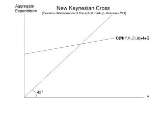
Income-expenditure line Aggregate expenditure(trillions of dollars) Income-expenditure line 450 0 Real GDP(trillions of dollars) At every point on this line, planned spending is equal to real GDP—so unplanned investment is zero
Actual versus planned investment Haley’s Hammers 2007 Investment Plans Planned spending for new plant and equipment . . . . . . . . . . . . . . . . . . . . . .$95,000 Planned inventory investment . . . . . . . . . . . . . . . . .0 Actual inventory investment . . . . . . . . . . . . . .3,500 Actual investment . . . . . . . . . . . .. . . . . . . . $98,500 Remember, that: Actual I = Planned I + Unplanned I
We normally cut back on production when we see our inventories piling up.
15.0 C+I+G+(X-M) 14.8 Real GDP demanded for a given price level is found where aggregate expenditure equals aggregate output – that is, where spending equals the amount produced, or real GDP. This occurs at point e, where the aggregate expenditure line intersects the 45-degree line. 14.0 Aggregate expenditure (trillions of dollars) d b e 13.2 c a 13.0 45° 0 13.0 14.0 Real GDP (trillions of dollars) 15.0 Deriving the real GDP demanded for a given price level
When Real GDP = $14 trillion • Planned spending of households, firms, government units, and foreigners is equal to real output; thus the plans of producing and spending units “match up.” • Firms on average experience zero unplanned investment. • Firms on average have nor reason to ‘scale up’ or ‘scale down’ production.
C+I+G+(X-M) C+I’+G+(X-M) 14.5 A $0.1 trillion increase in investment shifts the AE line up vertically by $0.1 trillion. Real GDP increases until it equals spending at point e’. As a result of the $0.1 trillion increase in investment, real GDP demanded increases by $0.5 trillion, to $14.5 trillion. 14.1 Aggregate expenditure (trillions of dollars) f h j e’ 14.0 k i e g 0.1 45° Real GDP (trillions of dollars) 0 14.0 14.1 14.5 The economy is initially at point e, where spending=real GDP demanded = $14.0 trillion. Effect of an increase in investment on real GDP demanded
Tracking the rounds of spending following a $100 billion increase in investment (billions of dollars) Assume that MPC = 0.8 and MPS = 0.6
Simple spending multiplier (k) Note that:
(a) At the initial price level =130, the AE line identifies real GDP demanded of $14.0 trillion: point e on panel (b). AE’ (P=140) AE” (P=120) AE (P=130) At the higher price level of 140, the AE line shifts down to AE’, and real GDP demanded falls to $13.5 trillion: point e’ on panel (b). e’’ Aggregate expenditure (trillions of dollars) e e’ e’ e e’’ At the lower price level of 120, the AE line shifts up to AE’’, and real GDP demanded increases to $14.5 trillion: point e” on panel (b). (b) Price level 140 45° 130 Real GDP (trillions of dollars) 0 13.5 14.0 14.5 Real GDP (trillions of dollars) 0 13.5 14.0 14.5 Connecting e, e’, and e’’ yields the downward-sloping AD curve. 120 AD The income-expenditure approach and the AD curve
(a) A shift of the AE line at a given price level shifts the AD curve. In (a), an increase in investment of $0.1 trillion, with the price level constant at 130, causes the aggregate expenditure line to increase from C+I+G+(X-M) to C+I’+G+(X-M). As a result, real DGP demanded increases from $14.0 trillion to $14.5 trillion. In (b), the aggregate demand curve has shifted from AD to AD’. At the prevailing price level of 130, real GDP demanded has increased by $0.5 trilion. 0.1 C+I’+G+(X-M) C+I+G+(X-M) e’ Aggregate expenditure (trillions of dollars) e e’ e (b) Price level 45° 130 Real GDP (trillions of dollars) 0 14.0 14.5 Real GDP (trillions of dollars) 0 14.0 14.5 AD’ AD A shift of AE line that shifts the AD curve
C+I’+G+(X-M) An increase in investment, other things constant, shifts the spending line up from C+I+G+(X-M) to C+I’+G+(X-M), increasing the quantity of real GDP demanded. C+I+G+(X-M) Aggregate expenditure (trillions of dollars) e’ e $0.1 45° Real GDP (trillions of dollars) 14.333 0 14.0 Effect of a shift of autonomous spending on real GDP demanded