Aggregate Expenditure
Macroeconomics for business

Aggregate Expenditure
E N D
Presentation Transcript
Aggregate Expenditure CHAPTER-3
CHAPTER CONTENTS • Actual Vs. Planned Expenditure • Autonomous Versus Induced Expenditure • Consumption And Saving Functions • MPC, MPS And Multiplier • Investment Spending • Government Spending • Export Earnings And Import Expenditure • Equilibrium In Two-, Three-, And Four- Sector Model • Expenditure Multipliers: Simple Multiplier, Investment Multiplier And Foreign Trade Multiplier
Aggregate Expenditure • The aggregate expenditure is the sum of all the expenditures undertaken in the economy by the factors during a specific time period. • The equation is: AE = C + I + G + NX. • The aggregate expenditure determines the total amount that firms and households plan to spend on goods and services at each level of income. • The aggregate expenditure is one of the methods that is used to calculate National Income or Gross Domestic Product(GDP) • When there is excess supply over the expenditure, there is a reduction in either the prices or the quantity of the output which reduces the total output (GDP) of the economy. • When there is an excess of expenditure over supply, there is excess demand which leads to an increase in prices or output (higher GDP).
Components of Aggregate Expenditure • Aggregate expenditure for final goods and services equals the sum of • Consumption expenditure, C • Investment, I • Government purchases of goods and services, G • Net exports, NX Thus:Aggregate expenditure = C + I + G + NX
Planned Vs Unplanned Investment • Investment has two components: • Planned investment as determined by investment demand schedule • Unplanned investment is unintended changes in the level of inventories • Actual investment = sum of planned and unplanned investment • At equilibrium: Unplanned investment = zero
Aggregate expenditure is the sum of Consumption expenditure (C), Investment (I), Government expenditure (G), Net export (NX) [Export (X) minus Import (M)] Note: Y is real GDP 8
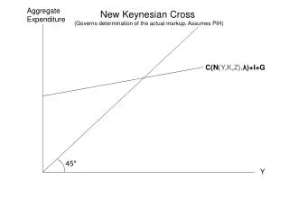
EQUILIBRIUM EXPENDITURE • Equilibrium expenditure is the level of aggregate expenditure when aggregate planned expenditure equals real GDP. • Equilibrium expenditure equals the real GDP at which the AE curve intersects the 45 line. • In macroeconomics, equilibrium in the goods market is the point at which planned aggregate expenditure is equal to aggregate output
EQUILIBRIUM EXPENDITURE • When aggregate planned expenditure exceeds real GDP, an unplanned decrease in inventories occurs. • When aggregate planned expenditure is less than real GDP, an unplanned increase in inventories occurs. • When aggregate planned expenditure equals real GDP, there are no unplanned inventories and real GDP remains at equilibrium expenditure
When aggregate planned expenditure is less than real GDP, firms cut production. Real GDP decreases. • When real GDP decreases, aggregate planned expenditure decreases. But real GDP decreases by more than planned expenditure, so eventually the gap between planned expenditure and actual expenditure closes. Vice a Versa
Equilibrium National Income • …is that level of national income where planned aggregate expenditure equals actual national income. Planned expenditure 45° line or actual expenditure Desired expenditure line E Actual National income
Autonomous versus induced Expenditure • Autonomous expenditure: Includes the components of aggregate expenditure that do not change when real GDP changes . • Induced expenditure: Includes the components of aggregate expenditure that change when real GDP changes.
Consumption (C) And Investment (I) • In a two sector model, a simple but an imaginary assumption of no government and no foreign trade is made. • Here Yd =C+S or Yd =AD (aggregate demand) • This also implies that C+S=C+I
Consumption “Consumption is the sole end and purpose of all production.” Adam Smith • Consumption is the act of spending income for buying goods and services to satisfy wants. • Determinants of consumption : • Disposable Income (after tax income) of the consumers(Yd) • Accumulated wealth or assets of consumers(W) • Expected future income, of Consumers(Ce) • The actual price level(P) • The expected general price level, Rate of interest(Pe) • Thriftiness,(T) • Age(A) • Sex(S) • Family size (Fs).
Classical Consumption Function • A relation between consumption and its various determinants is called the consumption function. • The consumption function taking all these determinants into account can be written as: C=f (Yd, W, Ye, P, Pe, r,A, s, FS…..)
Keynesian Consumption Function • Keynes, however, asserts that income alone is the most important determinant of consumption. Here, income refers to the disposable income. The Keynesian consumption function, thus, can be written as: • C=f (Yd), 1>f>0 • Where, C=Consumption demand Yd=Disposable income= (Y-T) Y=Personal income T=Taxes (related to income)
Keynesian Consumption Function • The assumption of the Keynesian consumption function is that consumption depends on income, other things being equal. The higher the income, higher is the consumption, ceteris paribus. • Keynes’ psychological law of consumption (The concept of the marginal propensity to consume). • Keynes argue that when the income increases, consumption also increases but not to the same extent as the increase in income.
Keynesian Psychological Law of Consumption “ The fundamental psychological law states that men are disposed of, as a rule and on the average, to increase their consumption as their income increases, but not by as much as the increase in their income.” • The idea is that when the income increases, consumption also increases but less than proportionately. Alternatively, Marginal Propensity To Consume (MPC) is positive but less than unity (0<MPC<1).
Marginal Propensity To Consume(MPC) • Keynesian Psychological Law is also called the MPC. • Given the consumption function: C= f (Yd), the MPC is the ratio between change in consumption expenditure and the change in income level. • MPC=∆C = Change in consumption ∆YdChange in disposable income • i.e. 0< =∆C <1 ∆Yd
Marginal Propensity to Consume • Suppose, initial income level is Rs. 1000 and consumption demand is Rs. 800. When income level increases to Rs. 1500, and consumption demand to Rs. 1200, MPC will be: • =∆C/ ∆Yd =400/500=0.80 • This implies that when income increases by Rs. 100, consumption demand increases by Rs 80. And the difference Rs. 20 is the saving. • This means Yd = C+S • i.e. Disposable income=Consumption+Saving
MPC in Consumption Function Equation • Short run Keynesian consumption function is often written as: C=Ca+bYd • Cais autonomous consumption function. This implies that Cais not related toincome level (Yd) since a minimum level of consumption is required just for survival even if there is no income. • And “b” is MPC in the above equation.
Average Propensity to Consume • The fraction of total disposable income spent on consumption demand is called the average propensity to consume (APC). • APC= Consumption demand = C Disposable income Yd • APC implies the average spending tendency of the community or the people of a country. • Given the consumption function, C=Ca+bYd • APC=C/Yd=Ca+bYd/Yd • Or, APC = C Yd
Main Observations • When disposable income increases, consumption also increases but not proportionately. • When disposable income increases, APC declines. • When disposable income increases, MPC remains constant and APC>MPC. • At low level of income, there is dissaving and at higher level of income there is saving. • At particular level of income (i.e. at Rs. 400, C=Yd), saving is just zero. This point is called the break even point.
Graphical Presentation Y-Axis C,S 45° line (Y=C+S) S=50 C E S=-50 C=Y=400 Ca=100 200 600 400 Disposable income (Yd )
Short Run And Long Run Consumption CLR: Consumption in the long run C=bYd Y-Axis C,S CSR : Consumption in the short run C=Ca+bYd Ca Disposable income (Yd )
Short Run And Long Run Consumption • The short run consumption is non-proportional in the sense that consumption is partly autonomous and partly induced that is related to the current disposable income. • The long run consumption fully depends on income. The long run autonomous consumption is zero and according to Keynes, in the long run, we all die if fail to generate our own income.
Saving Function • The part of the disposable income not spent on consumption is called saving. Saving is the difference between disposable income and consumption. • It is based on the premise that Yd=C+S • Then S=Yd-C • S=Yd- (Ca+bYd) • Or, S= -Ca+(1-b)Yd Where, -Ca=Autonomous saving that is negative or that is dis-saving. A person must borrow in order to survive. • 1-b is marginal propensity to save as we know b is marginal propensity to consume.
Saving Function • From the macroeconomic perspective, aggregate saving is that part of real output that is produced but not sold to consumers. Thus, aggregate saving is the sum total of the private saving, and government saving. • Gross National Saving=Govt. saving+ private saving • Personal saving is the difference between personal disposable income and the personal consumption expenditure. • Private saving is the sum of personal saving and gross business saving. Gross business saving is the profits minus dividends paid to individuals plus depreciation. • Government saving is the difference between government revenues and government expenditures.
Again To Remind: Types Of Saving private saving = (Y – T) – C public saving = T – G national saving, S = private saving + public saving = (Y –T ) – C + T – G = Y – C – G
Marginal Propensity To Save • MPS is the change in saving as a result of an additional unit of disposable income. • MPS =∆S = Change in saving ∆Yd Change in disposable income • Since MPC+MPS=1, when MPC increases, MPS decreases. This relationship between MPC and MPS can also be shown graphically by plotting MPS on the vertical axis and MPC on the horizontal axis. First think and draw yourself.
MPC+MPS=1 MPS S1 B1+s1=1 B2+s2=1 S2 O b1 b2 MPC
Average Propensity To Save • APS is the ratio between total saving and total disposable income. • APS =S = Saving Yd Disposable income • APS increases when disposable income increases and vice versa.
Graph For Saving Function S S E o Yd -Ca
Determinants of consumption and Saving • Since consumption is the counterpart of saving, both are related to each other. • Factors affecting the consumption demand also affect saving. • Thus, determinants of consumption and saving are interrelated and presented in the next slide.
Determinants of consumption and Saving • Change In Disposable Income Affects Consumption And Saving. • Once the Yd changes, both consumption and saving change. A higher Yd increases both C and S. • However, it also depends on the preference of an individual. • Increase in Yd shifts the budget line rightward indicating that more consumption and more saving are possible.
Determinants of consumption and Saving • Change In Interest Rate Affects Consumption And Saving. . • There is a positive relationship betweenrealinterest rate, r and saving, S. When r increases S also increases since r is the reward for saving. • Increase in r reduces consumption. Even people who borrow and consume are discouraged to consume more. • When there is more saving and less consumption due to increase in r, it is called the substitution effect of increased real interest rate.
Determinants of consumption and Saving • Change in price level and price expectations affect consumption and saving: • The effect of price level change on C and S depends on what happens to the real disposable income when price level changes. • If current disposable income rises or falls proportionately with the price level, real income remains unchanged. In this case, the shares of consumption and saving remain unchanged.
Determinants of consumption and Saving • Change in price level and price expectations affect consumption and saving: • Real income= nominal income/price level • For example, real income at present is current income/price level i.e. 2000/5=400 • After price level and Yd change say by 20 % i.e. 2400/6=400 • In both cases S and C remain unchanged since there is no change in real income.
Determinants of consumption and Saving • Change in price level and price expectations affect consumption and saving: • However, this may not be valid in the case of money illusion, a situation in which a person cares more about the nominal income than the real income. If a person increases his saving because of the money illusion than the real consumption will decline. • In the absence of money illusion, when real disposable income decreases because of the increase in price level, there will be an absolute decrease in real consumption expenditure.
Determinants of consumption and Saving • Change in price level and price expectations affect consumption and saving: • Given the disposable income, expectation of a higher price level in the future may cause increase in consumption expenditure thereby reducing the saving. Because higher price in the future period will reduce the value of saving in real term (value of money declines due to price rise). • If the expected price level declines, people postpone consumption expenditure and increase saving with the hope that they can take advantage of higher purchasing power of money they deposited.
Determinants of consumption and Saving 4. Pattern of income distribution: • According to N. Kaldor, people with low income level have higher MPC and hence lower MPS. On the contrary, people with higher income level have lower MPC and higher MPS. • This implies that MPS is higher for high income group and lower for low income group. In other words, low income group consumes whatever they earned while high income group saves more when income increases.
Determinants of consumption and Saving 4. Pattern of income distribution: • However, still there are debates. A number of hypothesis in discussion are : Absolute income hypothesis (J. M. Keynes) Relative income hypothesis (James Duesenberry) Permanent Income hypothesis (M. Friedman) Life-cycle hypothesis (F. Modigliani) • These are discussed in advanced level.
Determinants of consumption and Saving 5. Real assets, financial assets and outstanding debt affects consumption and saving: • Ceteris paribus, accumulation of wealth in terms of real (houses, other consumer durables) and financial (stocks, bonds, and other forms of deposit) assets leads to increase consumption expenditure. Given the size of real and financial assets, consumption expenditure depends on the rate of interest (as a return fro such assets) and the price level. • Any outstanding debt compels an individual to reduce consumption expenditure thereby saving more. In the case of no outstanding debt, this may be opposite.
Determinants of consumption and Saving 6. Thriftiness, old age security and social safety net also affect consumption and saving: • Attitudes toward thrift (desire to save more) also influences the allocation of disposable income between consumption and saving. If people are thriftier, they keep aside increasing fraction of their disposable income for future consumption by reducing current consumption. • In a society with sufficient provision of old-age security and social safety net, people will save less and consume more. Converse will hold in the absence of such program in the society.