Prof. David R. Jackson
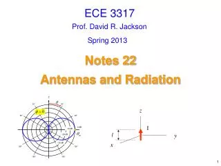
ECE 3317. Prof. David R. Jackson. Spring 2013. Notes 22 Antennas and Radiation . Antenna Radiation. +. -. We consider here the radiation from an arbitrary antenna. S. z. r. y. "far field". x. The far-field radiation acts like a plane wave going in the radial direction.

Prof. David R. Jackson
E N D
Presentation Transcript
ECE 3317 Prof. David R. Jackson Spring 2013 Notes 22 Antennas and Radiation
Antenna Radiation + - We consider here the radiation from an arbitrary antenna. S z r y "far field" x The far-field radiation acts like a plane wave going in the radial direction.
Antenna Radiation (cont.) + - How far do we have to go to be in the far field? Sphere of minimum diameter D that encloses the antenna. r This is justified from later analysis.
Antenna Radiation (cont.) z z S H y S E H y x E x The far-field has the following form: TMz TEz Depending on the type of antenna, either or both polarizations may be radiated (e.g., a vertical wire antenna radiates only TMz polarization.
Antenna Radiation (cont.) The far-field Poynting vector is now calculated:
Antenna Radiation (cont.) Hence we have or Note: In the far field, the Poynting vector is pure real (no reactive power flow).
Radiation Pattern The far field always has the following form: In dB:
Radiation Pattern (cont.) 30° 30° 60° 60° 0 dB -10 dB -20 dB -30 dB 120° 120° 150° 150° The far-field pattern is usually shown vs. the angle (for a fixed angle ) in polar coordinates. The subscript “m” denotes the beam maximum. A “pattern cut”
Radiated Power The Poynting vector in the far field is The total power radiated is then given by Hence we have
Directivity The directivity of the antenna in the directions (, ) is defined as The directivity in a particular direction is the ratio of the power density radiated in that direction to the power density that would be radiated in that direction if the antenna were an isotropic radiator (radiates equally in all directions). In dB, Note: The directivity is sometimes referred to as the “directivity with respect to an isotropic radiator.”
Directivity (cont.) The directivity is now expressed in terms of the far field pattern. Hence we have Therefore,
Directivity (cont.) 30° 30° z +h 60° 60° 0 dB feed -6 -3 -9 y 120° 120° x -h 150° 150° Two Common Cases Short dipole wire antenna (l << 0): D = 1.5 Resonant half-wavelength dipole wire antenna (l = 0 / 2): D = 1.643 Short dipole
Beamwidth The beamwidth measures how narrow the beam is. (the narrower the beamwidth, the higher the directivity). HPBW = half-power beamwidth
Sidelobes The sidelobe level measures how strong the sidelobes are. In this example the sidelobe level is about -13 dB Main beam Sidelobe level Sidelobes Sidelobes
Gain and Efficiency The radiationefficiency of an antenna is defined as Prad= power radiated by the antenna Pin= power input to the antenna The gain of an antenna in the directions (, ) is defined as In dB, we have
Gain and Efficiency (cont.) The gain tells us how strong the radiated power density is in a certain direction, for a given amount of input power. Recall that Therefore, in the far field:
Infinitesimal Dipole z I l y x The infinitesimal dipole current element is shown below. The dipole moment (amplitude) is defined as Il. The infinitesimal dipole is the foundation for many practical wire antennas. From Maxwell’s equations we can calculate the fields radiated by this source (e.g., see Chapter 7 of the Shen and Kong textbook).
Infinitesimal Dipole (cont.) The exact fields of the infinitesimal dipole in spherical coordinates are
Infinitesimal Dipole (cont.) In the far field we have: Hence, we can identify
Infinitesimal Dipole (cont.) The radiation pattern is shown below. 30° 30° 45o 60° 60° 0 dB -9 -6 -3 120° 120° HPBW = 90o 150° 150°
Infinitesimal Dipole (cont.) The directivity of the infinitesimal dipole is now calculated Hence
Infinitesimal Dipole (cont.) Evaluating the integrals, we have Hence, we have
Infinitesimal Dipole (cont.) 30° 30° 60° 60° 0 dB -9 -6 -3 120° 120° 150° 150° The far-field pattern is shown, with the directivity labeled at two points.
Wire Antenna A center-fed wire antenna is shown below. z +h I(z) vs. z I(z) Feed I0 y x -h A good approximation to the current is:
Wire Antenna (cont.) A sketch of the current is shown below for two cases. +h +h l I0 I0 l -h -h Resonant dipole (l = 0 / 2, k0h = /2) Short dipole (l <<0) Use
Wire Antenna (cont.) +h l -h Short Dipole The average value of the current is I0/2. I0 Infinitesimal dipole: Short dipole (l <<0 / 2) Short dipole:
Wire Antenna (cont.) z +h R r dz' z' Feed y x -h For an arbitrary length dipole wire antenna, we need to consider the radiation by each differential piece of the current. Far-field observation point I(z') Infinitesimal dipole: Wire antenna:
Wire Antenna (cont.) z R +h r dz' Feed y x -h Far-field observation point
Wire Antenna (cont.) z R +h r dz' Feed y x -h Far-field observation point It can be shown that this approximation is accurate when Note:
Wire Antenna (cont.) z R +h r dz' Feed y x -h Far-field observation point Hence we have
Wire Antenna (cont.) We define the array factor of the wire antenna: We then have the following result for the far-field pattern of the wire antenna: The term in front of the array factor is the far-field pattern of the unit-amplitude infinitesimal dipole.
Wire Antenna (cont.) Using our assumed approximate current function we have Hence The result is (derivation omitted)
Wire Antenna (cont.) In summary, we have Thus, we have
Wire Antenna (cont.) For a resonant half-wave dipole antenna The directivity is
Wire Antenna (cont.) Results
Wire Antenna (cont.) Radiated Power: Simplify using
Wire Antenna (cont.) Performing the integral gives us After simplifying, the result is then
Wire Antenna (cont.) z +h I(z) Feed y x -h The radiation resistance is defined from Circuit Model I0 I0 Z0 Zin For a resonant antenna (l 0 / 2), Xin = 0.
Wire Antenna (cont.) The radiation resistance is now evaluated. Using the previous formula for Prad, we have l0 /2 Dipole:
Wire Antenna (cont.) The result can be extended to the case of a monopole antenna I(z) h Feeding coax (see the next slide)
Wire Antenna (cont.) Vmonopole Vdipole I0 I0 + + - - Virtual ground Dipole This can be justified as shown below.
Receive Antenna + Einc VTh - l = 2h ZTh VTh + - The Thévenin equivalent circuit of a wire antenna being used as a receive antenna is shown below.
Example ZTh VTh + - Two lossless resonant half-wavelength vertical dipole wire antennas z Receive Transmit Prad[W] + r VTh x - Prad Receive Thévenin circuit Find the Thévenin voltage (magnitude of it).
Example (cont.) Design equations: Hence we have
Example (cont.) 73 [] 3.00 [mV] + - Assume these values: f = 1 [GHz] (0 = 29.979 [cm]) Prad = 10 [W] r = 1 [km] The result is Receive Thévenin circuit
Example (cont.) + - Next, calculate the power received by an optimum conjugate-matched load ZTh VTh For resonant antennas:
Effective Area + - Another way to characterize an antenna is with the effective area. This is more general than effective length (which only applies to wire antennas). Receive circuit: Assume an optimum conjugate-matched load: ZTh PL = power absorbed by load VTh Aeff= effective area of antenna (depends on incident angles) Pinc= average power density incident on antenna [W/m2]
Effective Area (cont.) We have the following general formula*: G(,) = gain of antenna in direction (,) *A poof is given in the Antenna Engineering book: C. A. Balanis, Antenna Engineering, 3rd Ed., 2055, Wiley.
Effective Area (cont.) Effective area of a lossless resonant half-wave dipole antenna Assuming normal incidence (= 90o): Hence
Effective Area (cont.) Example Find the receive power in the example below, assuming that the receiver is now connected to an optimum conjugate-matched load. f = 1 [GHz] (0 = 29.979 [cm]) Prad = 10 [W] r = 1 [km] z Receive Transmit Prad[W] r x Prad