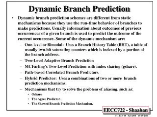
Dynamic Branch Prediction
Dynamic Branch Prediction. Marco D. Santambrogio: marco.santambrogio@polimi.it Simone Campanoni: xan@eecs.harvard.edu. Outline. Branch Prediction Techniques Dynamic Branch Prediction Performance of Branch Schemes. Dynamic Branch Prediction.


Dynamic Branch Prediction
E N D
Presentation Transcript
Dynamic Branch Prediction Marco D. Santambrogio: marco.santambrogio@polimi.it Simone Campanoni: xan@eecs.harvard.edu
Outline Branch Prediction Techniques Dynamic Branch Prediction Performance of Branch Schemes
Dynamic Branch Prediction Basic Idea: To use the past branch behavior to predict the future. We use hardware to dynamically predict the outcome of a branch: the prediction will depend on the behavior of the branch at run time and will change if the branch changes its behavior during execution. We start with a simple branch prediction scheme and then examine approaches that increase the branch prediction accuracy.
Dynamic Branch Prediction Schemes Dynamic branch prediction is based on two interacting mechanisms: Branch Outcome Predictor: To predict the direction of a branch (i.e. taken or not taken). Branch Target Predictor: To predict the branch target address in case of taken branch. These modules are used by the Instruction Fetch Unit to predict the next instruction to read in the I-cache. If branch is not taken PC is incremented. If branch is taken BTP gives the target address
Branch History Table Branch History Table (or Branch Prediction Buffer): Table containing 1 bit for each entry that says whether the branch was recently taken or not. Table indexed by the lower portion of the address of the branch instruction. Prediction: hint that it is assumed to be correct, and fetching begins in the predicted direction. If the hint turns out to be wrong, the prediction bit is inverted and stored back. The pipeline is flushed and the correct sequence is executed. The table has no tags (every access is a hit) and the prediction bit could has been put there by another branch with the same low-order address bits: but it doesn’t matter. The prediction is just a hint!
Branch History Table n-bit Branch Address BHT 2k entries k-bit Branch Address T/NT
Accuracy of the Branch History Table A misprediction occurs when: The prediction is incorrect for that branch or The same index has been referenced by two different branches, and the previous history refers to the other branch. To solve this problem it is enough to increase the number of rows in the BHT or to use a hashing function (such as in GShare).
1-bit Branch History Table Shortcoming of the 1-bit BHT: In a loop branch, even if a branch is almost always taken and then not taken once, the 1-bit BHT will mispredict twice (rather than once) when it is not taken. That scheme causes two wrong predictions: At the last loop iteration, since the prediction bit will say taken, while we need to exit from the loop. When we re-enter the loop, at the end of the first loop iteration we need to take the branch to stay in the loop, while the prediction bit say to exit from the loop, since the prediction bit was flipped on previous execution of the last iteration of the loop. For example, if we consider a loop branch whose behavior is taken nine times and not taken once, the prediction accuracy is only 80% (due to 2 incorrect predictions and 8 correct ones).
1-bit Branch History Table n-bit Branch Address 1-BHT 0 0 0 1 2k entries k-bit Branch Address 0 1 T/NT 1 1
2-bit Branch History Table The prediction must miss twice before it is changed. In a loop branch, at the last loop iteration, we do not need to change the prediction. For each index in the table, the 2 bits are used to encode the four states of a finite state machine.
2-bit Branch History Table n-bit Branch Address 2-BHT 00 01 10 2k entries (twice the memory used for the 1-BHT) 11 Keeping k-bit Branch Address 01 11 T/NT 11 01
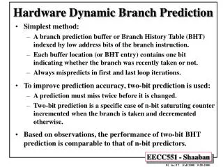
n-bit Branch History Table Generalization: n-bit saturating counter for each entry in the prediction buffer. The counter can take on values between 0 and 2n-1 When the counter is greater than or equal to one-half of its maximum value (2n-1), the branch is predicted as taken. Otherwise, it is predicted as untaken. As in the 2-bit scheme, the counter is incremented on a taken branch and decremented on an untaken branch. Studies on n-bit predictors have shown that 2-bit predictors behave almost as well.
Accuracy of 2-bit Branch History Table For IBM Power architecture executing SPEC89 benchmarks , a 4K-entry BHT with 2-bit per entry results in: Prediction accuracy from 99% to 82% (i.e. misprediction rate from 1% to 18%) Almost similar performance with respect to an infinite buffer with 2-bit per entry.
Correlating Branch Predictors The 2-bit BHT uses only the recent behavior of a single branch to predict the future behavior of that branch. Basic Idea: the behavior of recent branches are correlated, that is the recent behavior of other branches rather than just the current branch (we are trying to predict) can influence the prediction of the current branch.
Example of Correlating Branches subi r3,r1,2 bnez r3,L1; bb1 add r1,r0,r0 L1: subi r3,r2,2 bnez r3,L2; bb2 add r2,r0,r0 L2: sub r3,r1,r2 beqz r3,L3; bb3 L3: If(a==2) a = 0; bb1 L1: If(b==2) b = 0; bb2 L2: If(a!=b) {}; bb3 Branch bb3 is correlated to previous branches bb1 and bb2. If previous branches are both not taken, then bb3 will be taken(a!=b)
Correlating Branch Predictors Branch predictors that use the behavior of other branches to make a prediction are called Correlating Predictors or 2-level Predictors. Example a (1,1) Correlating Predictors means a 1-bit predictor with 1-bit of correlation: the behavior of last branch is used to choose among a pair of 1-bit branch predictors.
Correlating Branch Predictors: Example T1: Branch History Table if last branch taken T2: Branch History Table if last branch not taken Branch Address Last Branch Result Branch Prediction
Correlating Branch Predictors Record if the k most recently executed branches have been taken o not taken. The branch is predicted based on the previous executed branch by selecting the appropriate 1-bit BHT: One prediction is used if the last branch executed was taken Another prediction is used if the last branch executed was not taken. In general, the last branch executed is not the same instruction as the branch being predicted (although this can occur in simple loops with no other branches in the loops).
(m, n) Correlating Branch Predictors In general (m, n) correlating predictor records last m branches to choose from 2m BHTs, each of which is a n-bit predictor. The branch prediction buffer can be indexed by using a concatenation of low-order bits from the branch address with m-bit global history (i.e. global history of the most recent m branches).
(2, 2) Correlating Branch Predictors A (2, 2) correlating predictor has 4 2-bit Branch History Tables. It uses the 2-bit global history to choose among the 4 BHTs. Branch Address (k bit) 2k entries 2-bit global branch history 2-bit Prediction
Example of (2, 2) Correlating Predictor Example: a (2, 2) correlating predictor with 64 total entries 6-bit index composed of: 2-bit global history and 4-bit low-order branch address bits 4-bit branch address 24 entries 2-bit global branch history 2-bit Prediction
Example of (2, 2) Correlating Predictor Each BHT is composed of 16 entries of 2-bit each. The 4-bit branch address is used to choose four entries (a row). 2-bit global history is used to choose one of four entries in a row (one of four BHTs)
Branch Target Buffer Branch Target Buffer (Branch Target Predictor) is a cache storing the predicted branch target address for the next instruction after a branch We access the BTB in the IF stage using the instruction address of the fetched instruction (a possible branch) to index the cache. Typical entry of the BTB: The predicted target address is expressed as PC-relative
Structure of a Branch Target Buffer PC of fetched instruction Associative lookup Predicted target address Use lowest bits Of the PC Need also some validity bits No, instruction is not predicted To be a branch, proceed normally = Yes, instruction is a branch, PC should be used as next PC
Structure of a Branch Target Buffer BTB entry: Tag + Predicted target address (expressed as PC-relative for conditional branches) + Prediction state bits as in a Branch Outcome Predictor (optional). PC Tag Target Stat. T-T-NT = Target Address Present T/NT • In the BTB we need to store the predicted target address only for taken branches.
Speculation Without branch prediction, the amount of parallelism is quite limited, since it is limited to within a basic block – a straight-line code sequence with no branches in except to the entry and no branches out except at the exit. Branch prediction techniques can help to achieve significant amount of parallelism. We can further exploit ILP across multiple basic blocks overcoming control dependences by speculating on the outcome of branches and executing instructions as if our guesses were correct. With speculation, we fetch, issue and execute instructions as if out branch predictions were always correct, providing a mechanism to handle the situation where the speculation is incorrect. Speculation can be supported by the compiler or by the hardware.
References An introduction to the branch prediction problem can be found in Chapter 3 of: J. Hennessy and D. Patterson, “Computer Architecture, a Quantitative Approach”, Morgan Kaufmann, third edition, May 2002. A survey of basic branch prediction techniques can be found in:D. J. Lalja, “Reducing the Branch Penalty in Pipelined Processors”, Computer, pages 47-55, July 1988. A more detailed and advanced survey of the most used branch predictor architectures can be found in: M. Evers and T.-Y. Yeh, “Understanding Branches and Designing Branch Predictors for High-Performance Microprocessors”, Proceedings of the IEEE, Vol. 89, No. 11, pages 1610-1620, November 2001.