Accurate energy functionals for evaluating electron correlation energies
560 likes | 706 Vues
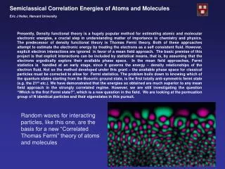
This work explores the development of accurate energy functionals for assessing electron correlation energies within quantum mechanics. It covers a historical context, theoretical foundations, and practical examples like the homogeneous electron gas and metal slabs. Key milestones in the discovery and development of quantum mechanics are highlighted, including major achievements by physicists such as J.J. Thompson and Niels Bohr. Additionally, it discusses various contemporary methods such as Configuration Interaction, Quantum Monte Carlo, and Kohn-Sham Density Functional Theory, emphasizing their applications in modern computational materials science.

Accurate energy functionals for evaluating electron correlation energies
E N D
Presentation Transcript
Accurate energy functionals for evaluating electron correlation energies 鄭載佾 國家理論科學研究中心物理組, 新竹‧
Outline (提綱) • History and context. • Theory. • Example 1. Homogeneous Electron Gas. • Example 2. Metal slabs. • Conclusions and perspectives. +
Discovery of the electron 1897 Could anything at first sight seem more impractical than a body which is so small that its mass is an insignificant fraction of the mass of an atom of hydrogen? J.J. Thompson (1856-1940) discovers the electron. (Cambridge, UK) Nobel Prize in Physics, 1906
Advent of new physics 1900 Quantization of energy Nobel Prize in Physics, 1918 1905 Photoelectric effect Nobel Prize in Physics, 1921 M. Planck (1858-1947)
1909 Measurement of electron charge and photoelectric effect. Nobel Prize in Physics, 1923 Robert Millikan (1868-1953) 1911 Disintegration of radiactive elements Nobel Prize in Chemistry, 1908
Development of quantum mechanics 1913 Quantum theory of the atom. Nobel Prize in Physics, 1922 Niels Bohr (1885-1962)
Paul Dirac (1902-1984) 1938 Development of quantum mechanics 1921 1925 1929 Statistical mechanics of electrons W. Pauli (1900-1958) 1945 E. Fermi (1901-1954) 1938 Louis De Broglie (1892-1987)
Development of quantum mechanics 1926 1932 1933 W. Heisenberg (1901-1976) Erwin Schrodinger (1887-1961)
Applications in solids 1928 1952 Forbidden region Felix Bloch 1905-1983
First attempts in electronic structre calculation • Egil Hylleraas. Configuration interaction, correlated basis functions. • Douglas Hartree and Vladimir Fock. Mean field calculations. • Wigner and Seitz. Cellular method. 1928 - 1932
More milestones (According to D. Pines) • Bohr & Mottelson. Collective model of nucleus. (1953) • Bohm & Pines. Random Phase Approximation. (1953) • Gell-Mann & Brueckner. Many body perturbation theory. (1957)
More milestones (According to P. Coleman) • BCS theory of superconductivity. • Renormalization group. • Quantum hall effect, integer and fractionary. • Heavy fermions. • High temperature superconductivity.
More is different “At each level of complexity, entirely new properties appear, and the understanding of these behaviors requires research which I think is as fundamental in its nature as any other” P. W. Anderson. Science, 177:393, 1972.
Theory First principles electronics structure calculation
Quotation from H. Lipkin “We can begin by looking at the fundamental paradox of the many-body problem; namely that people who do not know how to solvethe three-body problem are trying to solve the N-body problem. Our choice of wave functions is very limited; we only know how to use independent particle wave functions. The degree to which this limitation has invaded our thinking is marked by our constant use of concepts which have meaning only in terms of independent particle wave functions: shell structure, the occupation number, the Fermi sea and the Fermi surface, the representation of perturbation theory by Feynman diagrams. All of these concepts are based upon the assumption that it is reasonable to talk about a particular state being occupied or unoccupied by a particle independently of what the other particles are doing. This assumption is generally not valid, because there are correlations between particles. However, independent particle wave functions are the only wave functions that we know how to use. We must therefore find some method to treat correlations using these very bad independent particle wave functions.” Annals of Physics 8, 272 (1960)
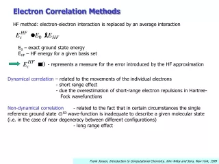
Currently available methods • Configuration Interaction. Quantum Monte Carlo. (Wave function) • Many-body perturbation theory. (Green’s function) • Kohn-Sham Density Functional Theory (Density).
Currently available methods • Configuration Interaction. Quantum Monte Carlo. (Wave function) • Many-body perturbation theory. (Green’s function) • Kohn-Sham Density Functional Theory (Density).
Many-body theory • Electronic and optical experiments often measure some aspect of the one-particle Green’s function • The spectral function, Im G, tells you about the single-particle-like approximate eigenstates of the system: the quasiparticles • Can formulate an iterative expansion of the self-energy S in powers of W, the screened Coulomb interaction, the leading term of which is the GW approximation • Can now perform such calculations computationally for real materials, without adjustable parameters. +
Currently available methods • Configuration Interaction. Quantum Monte Carlo. (Wave function) • Many-body perturbation theory. (Green’s function) • Kohn-Sham Density Functional Theory (Density).
KS-DFT formalism • It provides an independent particle scheme that describes the exact ground state density and energy.
KS-DFT formalism • Given the KS orbitals of the system we have.
KS-DFT formalism • The effective potential associated to the fictitious system is
The effective potential associated to the fictitious system is KS-DFT formalism • The effective potential associated to the fictitious system is
Homogeneous Electron Gas Independent electron approximation
Correlation energy • RPA. Bohm and Pines. (1953) • Gell-Mann and Brueckner. ( 1957) • Sawada. (1957) • Hubbard. (1957) • Nozieres and Pines. (1958) • Quinn and Ferrel. (1958) • Ceperley and Alder. (1980) 此事古難全
Ground-state energy of HEG Phys. Rev. Lett. 45, 566 (1980)
Density-density response function. (or Polarization) RPA response function
Density-density response function. (or Polarization) Exact response function
Density-density response function. (or Polarization) Hubbard response function Hubbard local field factor
Hubbard vertex correction Considers the Coulomb repulsion between electrons with antiparallel spins.
Many-body effects Local field factor ~ TDDFT fxc kernel Let’s remember that
Approximations for fxc • The simplest form is ALDA • But it gives too poor energy when used with the ACFD formula. Reminder
HEG Correlation energies Phys. Rev. B 61, 13431, (2000)
Energy optimized kernels • Dobson and Wang. • Optimized Hubbard. where
Performance of kernels Phys. Rev. B 70, 205107 (2004)
One Jellium Slab Thickness L = 6.4rs
Two slabs • Binding energies. (mHa/elec) • Surface energies. (erg/cm2)
Interaction energies Thickness L = 3rs and rs = 1.25