Download
1 / 57
570 likes | 826 Vues
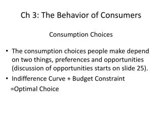
Ch 3: The Behavior of Consumers . Consumption Choices. The consumption choices people make depend on two things, preferences and opportunities (discussion of opportunities starts on slide 25). Indifference Curve + Budget Constraint =Optimal Choice. Preferences. Some Definitions

E N D
Ch 3: The Behavior of Consumers Consumption Choices • The consumption choices people make depend on two things, preferences and opportunities (discussion of opportunities starts on slide 25). • Indifference Curve + Budget Constraint =Optimal Choice
Preferences Some Definitions • Bundle: The collection of goods you consume (includes information on the quantity of each good too). • Utility: the economist’s term for how satisfied/happy you are. • Preferences: People’s feelings about how much utility they derive from different bundles. • Cardinal Measurement: The old way of thinking about utility. That utility, like height or temperature could be measured on a specific scale and would mean the same thing for everyone.
Ordinal Measurement • If someone tells us they prefer one bundle of goods to another, all we can say is the preferred bundle generates more utility. That is, we can order or rank the bundles in terms of how much utility they provide. If bundle A is preferred to bundle B is preferred to bundle C, we cannot tell whether the increase from moving from C to B is greater than the benefit from moving from B to A. • In addition, there is no way to make interpersonal comparisons of utility.
Modeling Preferences • For ease, we want to reduce the world into one in which consumers can only buy two goods. • We may not care where people’s preferences come from, but we do make some assumptions about their preferences. • To study people’s choices, we look at a Cartesian plane that contains every possible bundle. • Bundle A: 2 beers, 4 slices of pizza • Bundle B: 3 beers, 2 slices of pizza • A person has three preference options regarding these bundles. • A preferred to B • B preferred to A • Indifferent to A and B
Preference Assumptions • Completeness • Nonsatiation • Transitivity • Convexity
Completeness • All potential consumptions bundles are ranked. • Which means that for every two bundles on the graph, you have a definite opinion as to whether one is preferred to the other or you are indifferent.
Nonsatiation or “More is Better” • More of a good is preferred to less • Bundle C (2 beer and 5 slices of pizza) is preferred to A (2 beer and 4 slices), but not necessarily B (3 beer and 2 slices). • Bundle D (4 beer and 5 slices of pizza) is preferred to A, B and C
Transitivity • If C is preferred to A, and A is preferred to B, then C is preferred to B.
Convexity • Some of both goods is preferred to all of one good. • Likely that you prefer 1 hamburger, 1 fries, and 1 soda to 3 fries. • Likely that someone prefers 3 beers and 3 slices of pizza to 5 beers and 1 slice of pizza.
Convexity with a Graph If you draw a straight line connecting the axes, utility will tend to be higher at the mid point of the line than at the end points.
Implication of Convexity • If we have 20 shirts and 1 pair of pants, we are willing to trade 5 shirts for one more pair of pants to remain equally happy. • If we have 11 shirts and 9 pairs of pants, we are willing to trade one for one and will remain equally happy. • If we have 3 shirts and 17 pairs of pants, we are willing to trade 1 shirt for 8 more pairs of pants to remain equally happy.
With these few assumptions, we can build a graphical model of preferences. • First, draw vertical and horizontal lines through Bundle A. • Based on the nonsatiation and completeness assumptions, we can find areas on the graph with bundles that we know are either preferred (NE of A) or inferior to Bundle A (SW of A).
If we find all the bundles that are equally preferred to bundle A, we get a curve that represents all the equally preferred bundles.
Indifference Curve • Economists call this curve that contains all the equally preferred bundles the “Indifference Curve.”
Preference Assumptions and I-Curves • All bundles lie on one indifference curve (Completeness) • They are downward sloping and one that lies to the Northeast of another one generates more utility (Nonsatiation) • Two I-curves cannot cross (Transitivity and Nonsatiation would be violated if they did) • They become less steep as we move down to the right (Convexity).
Marginal Value (a.k.a. Marginal Rate of Substitution – MRS) • How much of good on y-axis are we willing to give up for one more unit of the good on the x-axis and remain indifferent? • That is, MRS tells us the marginal value of the good on the x-axis (1 beer) in terms of the other good, a slice of pizza. • It is equal to the slope of the I-curve. So, • MRS = Rise/Run = Pizza/Beer • The slope is negative, indicating that to remain indifferent, we give up some of one good when we get one more unit of the other.
Another Implication of Convexity • The MRS becomes smaller (and the indifference curve becomes flatter) as we consume more of the good on the x-axis. • That is, to remain indifferent, as we gain more of good on x-axis, we are willing to give up less of good on y-axis to gain one additional unit of good on x-axis.
Opportunities • Preferences are all about how we feel about the desirability of different bundles. • Opportunities are all about which bundles we can actually afford. • To choose the right bundle, we need both.
The Budget Constraint • Set of all affordable bundles given income and the price • Say we are choosing how many Tacos and Hamburgers to consume each week. • I: Weekly income • T: Quantity of tacos consumed • Pt: Price of Tacos • H: Quantity of hamburgers consumed • Ph: Price of Hamburgers • Budget Constraint: T*Pt + H*Ph = I (that is, total expenditure on both good must equal your income)
Dallas Water Pricing • What is the budget constraint for a consumer that buys water and some good Y (PY = $1). • Income is $200 • Price of water varies by consumption: • Pw = 0 for first 500 gallons • Pw = .10 for 500<W<1000 • Pw = .20 for W>1000
Start with W = 0 and determine how much X could be consumed, then figure out how this changes as W increases... Until you run out of income.
He says it so well in the text From Landsburg: • “The budget constraint conveys an entirely different kind of information than the indifference curves do. The indifference curves reflect the consumer’s preferences without regard to what he can actually afford to buy. The budget line show which baskets he can afford to buy (that is, it shows his opportuities) without regard to his preferences.
Finding the Optimal Bundle • To get the most utility, we must compare all the bundles on our budget constraint to find the one that yields the most utility. • As it turns out, the indifference curve that does not cross the budget constraint but only just touches it at one point will contain the best feasible bundle (at that point of tangency between the I-curve and the budget constraint). • Because it is a tangency, at the optimal bundle, the MRS (slope of I-curve) = Px/Py (the slope of the budget constraint).
If MRS > Px/Py, then what? • Take all actions (buy one more X) if the MB > MC • Px = 4, Py = 2, Px/Py = 2, so to get an extra X, you HAVE to give up 2 Y (MC of one more X = 2Y). • From A to C, MRS = 5, so to get an extra X, you are WILLING to give up 5 Y (MB of one more X is 5Y). • Therefore, consuming one more X sounds like a pretty good deal.
From A, to consume one more X, the person is willing to give up 5 units of Y (that is the MB of the 3rd x). But the 3rd X will only cost the person 2 Y. Therefore, the move allows a higher level of Utility.
As you consume another X, the MRS falls. So once you get to point B, the MRS is, say 3. Since you still HAVE to give up 2 Y for an X, and you are now willing to give up 3, it is still a good deal to consume one more X. So, moving from pt. B to E is a good move. At E, however, MRS = 2 and Px/Py =2. That is, what you have to pay for an additional unit of X (MC of X) and what you are willing to pay (MB of X) is the same.
The optimal bundle? • A person can keep making themselves better off as long as the willingness to pay (MB or Marginal Value or MRS) for an additional unit of X exceeds the MC (the true opportunity cost of consuming one more X). • At a tangency, the MB of one more X = MC of one more X and the highest level of utility is achieved.
Who is Thirstier? Bread Bread Jack and Jill each have 6 units of Bread and Water. But who values one additional unit of water more? Jill Jack 6 6 Water 6 6 Water
Who is Thirstier? • Answer: Jack, as at this same bundle of bread and water (B= 6, W = 6), his MRS is higher. • Next question: If bread costs $1 and water costs $2, whose MRS will be higher once Jack and Jill choose their optimal bundles?
Trick Question: Both will have the same MRS at their respective optimal bundles. Bread Bread When we draw in Budget Constraints with slopes of ½ for each of them and they find where their MRS = ½, Jack consumes more water and Jill consumes more bread than B = 6, W = 6. 6 Jill 6 Jack Water 6 6 Water
MRS = MRS = MRSbut X ≠ X ≠ X • So, facing the same prices, ALL consumers will have the same MRS at their optimal bundles, but for consumers with different preferences, they will all choose different quantities of all goods.
Some Non-standard Outcomes and Situations • Corner Solution • Perfect Compliments • Perfect Substitutes
Corner Solution: When does an optimal bundle not result in MRS = Px/Py? Tea • Corner Solution: When we SO prefer one good that given current prices, MRS > Px/Py even when we consume zero Y. (or, at the other corner, when MRS<Px/Py even when we consume zero X). Coffee
Perfect Substitutes: Goods that you view as identical Desani Water, 16 oz., d • Indifference curves will be straight lines. • Optimal bundle will be at a corner solution. I-curve in black, MRS = 1 MRS does not change along curve Blue budget line, Pd = 2, Pdb = 1, consume DB only Red budget line, Pd = 1, Pdb = 2, consume D only U1 Deja Blue Water, 16 oz., db
Perfect Compliments: Goods that are ALWAYS consumed together Whether the budget line is red or blue, the optimal bundle is 2 pairs of skis and 2 pairs of boots. A third pair of boots makes you no better off unless you get a 3rd pair of skis. • Optimal bundles will always be along a ray extending from the origin, Px/Py is irrelevant Pairs of Skis 2 U2 1 U1 1 Pairs of Ski Boots 2
Implications of the Model • If prices of all goods rise, you will be worse off. • If prices of all goods fall, you are better off. • But what if some prices rise and others fall? It is hard to say. • HOWEVER, if some prices rise and others fall in such a way that you can still consume the same bundle as before (while exhausting all income), then you will be better off. • This outcome actually has lots of policy consequences. • Let’s see how it works.
Initial Conditions • You eat two goods, Mangos and Apples. • I = $100. • Pm = $5/lb. • Pa = $4/lb. • M = 0, A = 25 • M= 20, A = 0 • Consume M = 12, A = 10 – total expenditure is $100.
Initial Optimal Bundle Apples I = $100. Pm = $5/lb. Pa = $4/lb. Consume M = 12, A = 10 25 10 Mangos 20 12
Is the Initial Optimal Bundle still affordable with new prices? Apples I = $100. Pm = $5$3 Pa = $4$6.40 Consume M = 12, A = 10 25 10 Mangos 20 12
Is the Initial Optimal Bundle still affordable with new prices? Apples I = $100, Pm = $5$3, Pa = $4$6.40. If M(=12)*$3+A(=10)*$6.40>100 Worse-off If M(=12)*$3+A(=10)*$6.40<100 Better-off 25 10 Mangos 20 12
Is the Initial Optimal Bundle still affordable with new prices? • We can still consume the same bundle, but is that optimal? Nope. Apples I = $100. Pm = $3/lb. Pa = $6.40/lb. Could Consume M = 12, A = 10 25 15.625 10 Mangos 33.33 20 12
Is the Initial Optimal Bundle still affordable with new prices? • With the blue budget line, we can consume more mangos and fewer apples and move to the red I-curve – which provides more utility. Apples I = $100. Pm = $3/lb. Pa = $6.40/lb. Consume M = 15, A = 8.6 25 15.625 10 8.6 Mangos 33.33 20 12 15
Utility Functions & Indiff. Curves x2 (2,3)(2,2)~(4,1) p U º 6 U º 4 x1
Utility Functions & Indiff. Curves 3D plot of consumption & utility levels for 3 bundles U(2,3) = 6 Utility U(2,2) = 4 U(4,1) = 4 x2 x1
Marginal Utility • Marginal Utility is the change in utility from consuming one more unit of a good. • U/X = MUx • In calculus, ∂U/∂X = MUx • If we consume only goods X and Y and our consumption bundle changes, the following must be true: X*MUx + Y*MUy = U • With the caveat that over the change in each good, MUx and MUy remains constant. This is only true for VERY small changes in X and Y. But that is why economists use calculus to work with the model – something we won’t be doing in this class.
Utility Held Constant The loss in utility from giving up 3 units of B = MUb*-3 The gain in utility from consuming an extra unit of C = MUc*1 Beets • Along an I-Curve, Utility does not change, so the change in utility from losing 3B is exactly offset by the gain from one more C. 8 X B=3 Y 5 U1 2 3 Cabbage C=1