Download
1 / 85
860 likes | 1.09k Vues
CSCE 580 Artificial Intelligence Ch.4: Informed (Heuristic) Search and Exploration. Fall 2008 Marco Valtorta mgv@cse.sc.edu. Acknowledgment. The slides are based on the textbook [AIMA] and other sources, including other fine textbooks and the accompanying slide sets

E N D
CSCE 580Artificial IntelligenceCh.4: Informed (Heuristic) Search and Exploration Fall 2008 Marco Valtorta mgv@cse.sc.edu
Acknowledgment • The slides are based on the textbook [AIMA] and other sources, including other fine textbooks and the accompanying slide sets • The other textbooks I considered are: • David Poole, Alan Mackworth, and Randy Goebel. Computational Intelligence: A Logical Approach. Oxford, 1998 • A second edition (by Poole and Mackworth) is under development. Dr. Poole allowed us to use a draft of it in this course • Ivan Bratko. Prolog Programming for Artificial Intelligence, Third Edition. Addison-Wesley, 2001 • The fourth edition is under development • George F. Luger. Artificial Intelligence: Structures and Strategies for Complex Problem Solving, Sixth Edition. Addison-Welsey, 2009
Outline • Informed = use problem-specific knowledge • Which search strategies? • Best-first search and its variants • Heuristic functions? • How to invent them • Local search and optimization • Hill climbing, local beam search, genetic algorithms,… • Local search in continuous spaces • Online search agents
Review: Tree Search function TREE-SEARCH(problem,fringe) return a solution or failure fringe INSERT(MAKE-NODE(INITIAL-STATE[problem]), fringe) loop do if EMPTY?(fringe) then return failure node REMOVE-FIRST(fringe) if GOAL-TEST[problem] applied to STATE[node] succeeds then return SOLUTION(node) fringe INSERT-ALL(EXPAND(node, problem), fringe) A strategy is defined by picking the order of node expansion
Best-First Search • General approach of informed search: • Best-first search: node is selected for expansion based on an evaluation functionf(n) • Idea: evaluation function measures distance to the goal. • Choose node which appears best • Implementation: • fringe is queue sorted in decreasing order of desirability. • Special cases: greedy search, A* search
Heuristics and the State-Space Search Heuristic Function • “A rule of thumb, simplification, or educated guess that reduces or limits the search for solutions in domains that are difficult and poorly understood.” • h(n)= estimated cost of the cheapest path from node n to goal node. • If n is goal thenh(n)=0
Romania with Step Costs in km • hSLD=straight-line distance heuristic. • hSLD can NOT be computed from the problem description itself
Greedy Best-first Search • Consider f(n)=h(n) • Expand node that is closest to goal = greedy best-first search
Greedy Search Example Arad (366) • Assume that we want to use greedy search to solve the problem of travelling from Arad to Bucharest. • The initial state=Arad
Greedy Search Example Arad Zerind(374) Sibiu(253) Timisoara (329) • The first expansion step produces: • Sibiu, Timisoara and Zerind • Greedy best-first will select Sibiu.
Greedy Search Example Arad Sibiu Arad (366) Rimnicu Vilcea (193) Fagaras (176) Oradea (380) • If Sibiu is expanded we get: • Arad, Fagaras, Oradea and Rimnicu Vilcea • Greedy best-first search will select: Fagaras
Greedy Search Example Arad Sibiu Fagaras Sibiu (253) Bucharest (0) • If Fagaras is expanded we get: • Sibiu and Bucharest • Goal reached !! • Yet not optimal (see Arad, Sibiu, Rimnicu Vilcea, Pitesti)
Properties of Greedy Search • Completeness: NO (cf. Depth-first search) • Check on repeated states • Minimizing h(n) can result in false starts, e.g. Iasi to Fagaras
Properties of Greedy Search • Completeness: NO (cfr. DF-search) • Time complexity? • Cf. Worst-case DF-search (with m maximum depth of search space) • Good heuristic can give dramatic improvement.
Properties of Greedy Search • Completeness: NO (cfr. DF-search) • Time complexity: • Space complexity: • Keeps all nodes in memory
Properties of Greedy Search • Completeness: NO (cfr. DF-search) • Time complexity: • Space complexity: • Optimality? NO • Same as DF-search
A* Search • Best-known form of best-first search • Idea: avoid expanding paths that are already expensive • Evaluation function f(n)=g(n) + h(n) • g(n) the cost (so far) to reach the node • h(n) estimated cost to get from the node to the goal • f(n) estimated total cost of path through n to goal
A* Search • A* search uses an admissible heuristic • A heuristic is admissible if it never overestimates the cost to reach the goal Formally: 1. h(n) <= h*(n) where h*(n) is the true cost from n 2. h(n) >= 0 so h(G)=0 for any goal G. e.g. hSLD(n) (the straight line heuristic) never overestimates the actual road distance
Uniform-Cost (Dijkstra) for Graphs Original Reference: Dijkstra, E. W. "A Note on Two Problems in Connexion with Graphs.“ Numerische Matematik, 1 (1959), 269-271 • 1. Put the start node s in OPEN. Set g(s) to 0 • 2. If OPEN is empty, exit with failure • 3. Remove from OPEN and place in CLOSED a node n for which g(n) is minimum; in case of ties, favor a goal node • 4. If n is a goal node, exit with the solution obtained by tracing back pointers from n to s • 5. Expand n, generating all of its successors. For each successor n' of n: • a. compute g'(n')=g(n)+c(n,n') • b. if n' is already on OPEN, and g'(n')<g(n'), let g(n')=g'(n’) and redirect the pointer from n' to n • c. if n' is neither on OPEN or on CLOSED, let g(n')=g'(n'), attach a pointer from n' to n, and place n' on OPEN • 6. Go to 2
A* 1. Put the start node s in OPEN. . 2. If OPEN is empty, exit with failure. . 3. Remove from OPEN and place in CLOSED a node n for which f(n) is minimum. 4. If n is a goal node, exit with the solution obtained by tracing back pointers from n to s. 5. Expand n, generating all of its successors. For each successor n' of n: a. Compute g'(n'); compute f'(n')=g'(n')+h(n') b. if n' is already on OPEN or CLOSED and g'(n')<g(n'), let g(n')=g'(n'), let f(n')=f'(n'), redirect the pointer from n' to n and, if n' is on CLOSED, move it to OPEN. c. if n' is neither on OPEN nor on CLOSED, let f(n')=f'(n'), attach a pointer from n' to n, and place n' on OPEN. 6. Go to 2.
A* with Monotone Heuristics 1. Put the start node s in OPEN. 2. If OPEN is empty, exit with failure. 3. Remove from OPEN and place in CLOSED a node n for which f(n) is minimum. 4. If n is a goal node, exit with the solution obtained by tracing back pointers from n to s. 5. Expand n, generating all of its successors. For each successor n' of n: a. Compute g'(n'); compute f'(n')=g'(n')+h(n') b. if n' is already on OPEN and g'(n')<g(n'), let g(n')=g'(n'), let f(n')=f'(n'), and redirect the pointer from n' to n. c. if n' is neither on OPEN nor on CLOSED, let f(n')=g'(n')+h(n'), g(n')=g'(n'), attach a pointer from n' to n, and place n' on OPEN. 6. Go to 2.
A* Search Example • Find Bucharest starting at Arad • f(Arad) = c(Arad,Arad)+h(Arad)=0+366=366
A* Search Example • Expand Arrad and determine f(n) for each node • f(Sibiu)=c(Arad,Sibiu)+h(Sibiu)=140+253=393 • f(Timisoara)=c(Arad,Timisoara)+h(Timisoara)=118+329=447 • f(Zerind)=c(Arad,Zerind)+h(Zerind)=75+374=449 • Best choice is Sibiu
A* Search Example • Expand Sibiu and determine f(n) for each node • f(Arad)=c(Sibiu,Arad)+h(Arad)=280+366=646 • f(Fagaras)=c(Sibiu,Fagaras)+h(Fagaras)=239+179=415 • f(Oradea)=c(Sibiu,Oradea)+h(Oradea)=291+380=671 • f(Rimnicu Vilcea)=c(Sibiu,Rimnicu Vilcea)+ h(Rimnicu Vilcea)=220+192=413 • Best choice is Rimnicu Vilcea
A* Search Example • Expand Rimnicu Vilcea and determine f(n) for each node • f(Craiova)=c(Rimnicu Vilcea, Craiova)+h(Craiova)=360+160=526 • f(Pitesti)=c(Rimnicu Vilcea, Pitesti)+h(Pitesti)=317+100=417 • f(Sibiu)=c(Rimnicu Vilcea,Sibiu)+h(Sibiu)=300+253=553 • Best choice is Fagaras
A* Search Example • Expand Fagaras and determine f(n) for each node • f(Sibiu)=c(Fagaras, Sibiu)+h(Sibiu)=338+253=591 • f(Bucharest)=c(Fagaras,Bucharest)+h(Bucharest)=450+0=450 • Best choice is Pitesti !!!
A* Search Example • Expand Pitesti and determine f(n) for each node • f(Bucharest)=c(Pitesti,Bucharest)+h(Bucharest)=418+0=418 • Best choice is Bucharest !!! • Optimal solution (only if h(n) is admissible) • Note values along optimal path !!
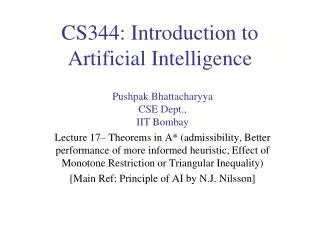
Admissible Heuristics and Search Algorithms • A heuristic h(n) is admissible if for every node n, h(n) ≤ h*(n), where h*(n) is the true cost to reach the goal state from n • An admissible heuristic never overestimates the cost to reach the goal, i.e., it is optimistic • Example: hSLD(n) (never overestimates the actual road distance) • A search algorithm is admissible if it returns an optimal solution path • [AIMA] calls such an algorithm optimal, instead of admissible • Theorem: If h(n) is admissible, A* (as presented in this set of slides) is admissible on graphs
Admissibility of A* • See Section 3.1.3 of: Judea Pearl. Heuristics: Intelligent Search Strategies for Computer Problem Solving. Addison-Wesley, 1984. • Especially Lemma 1 and Theorem 2 (pp. 77-78) • Note that admissibility of A* does not require monotonicity of the heuristics. [AIMA] claims otherwise on p.99. The confusion is probably due to the fact that admissibility only requires an optimal solution to be returned for a goal node (for which h=0), rather than for every node that is CLOSED • A* finds shortest paths to every node it closes with monotone (consistent) heuristics
Admissibility of A*: A Proof • The following proof is from [P]. Because of all the undefined terms, we should consider it a proof sketch. • The first path to a goal selected is an optimal path. The f-value for any node on an optimal solution path is less than or equal to the f-value of an optimal solution. This is because h is an underestimate of the actual cost from a node to a goal. Thus the f-value of a node on an optimal solution path is less than the f-value for any non-optimal solution. Thus a non-optimal solution can never be chosen while there is a node on the frontier that leads to an optimal solution (as an element with minimum f-value is chosen at each step). So before we can select a non-optimal solution, you will have to pick all of the nodes on an optimal path, including each of the optimal solutions.
Admissibility of A* • See Section 3.1.3 of: Judea Pearl. Heuristics: Intelligent Search Strategies for Computer Problem Solving. Addison-Wesley, 1984. • Especially Lemma 1 and Theorem 2 (pp. 77-78) • Note that admissibility of A* does not require monotonicity of the heuristics. [AIMA] claims otherwise on p.99. The confusion is probably due to the fact that admissibility only requires an optimal solution to be returned for a goal node (for which h=0), rather than for every node that is CLOSED • A* finds shortest paths to every node it closes with monotone (consistent) heuristics
Consistent Heuristics • A heuristic is consistent if for every node n, every successor n' of n generated by any action a, h(n) ≤ c(n,a,n') + h(n') • If h is consistent, we have f(n') = g(n') + h(n') = g(n) + c(n,a,n') + h(n') ≥ g(n) + h(n) = f(n) • i.e., f(n) is non-decreasing along any path • Theorem: If h(n) is consistent, A* never expands a node more than once
Optimality of A* on Graphs • A* expands nodes in order of increasing f value • Contours can be drawn in state space • Uniform-cost search adds circles. • F-contours are gradually Added: 1) nodes with f(n)<C* 2) Some nodes on the goal Contour (f(n)=C*) Contour I has all Nodes with f=fi, where fi < fi+1
A* search, evaluation • Completeness: YES • Time complexity: • Number of nodes expanded is still exponential in the length of the solution.
A* Search • Completeness: YES • Time complexity: (exponential with path length) • Space complexity: • It keeps all generated nodes in memory • Hence space is the major problem not time
A* search, evaluation • Completeness: YES • Time complexity: (exponential with path length) • Space complexity:(all nodes are stored) • Optimality: YES • Cannot expand fi+1 until fi is finished. • A* expands all nodes with f(n)< C* • A* expands some nodes with f(n)=C* • A* expands no nodes with f(n)>C* Also optimally efficient (not including ties)
Memory-bounded heuristic search • Some solutions to A* space problems (maintain completeness and optimality) • Iterative-deepening A* (IDA*) • Here cutoff information is the f-cost (g+h) instead of depth • Recursive best-first search(RBFS) • Recursive algorithm that attempts to mimic standard best-first search with linear space. • (simple) Memory-bounded A* ((S)MA*) • Drop the worst-leaf node when memory is full
Recursive best-first search function RECURSIVE-BEST-FIRST-SEARCH(problem) return a solution or failure return RFBS(problem,MAKE-NODE(INITIAL-STATE[problem]),∞) function RFBS( problem, node, f_limit) return a solution or failure and a new f-cost limit if GOAL-TEST[problem](STATE[node]) then return node successors EXPAND(node, problem) ifsuccessors is empty then return failure, ∞ for eachsinsuccessorsdo f [s] max(g(s) + h(s), f [node]) repeat best the lowest f-value node in successors iff [best] > f_limitthen return failure, f [best] alternative the second lowest f-value among successors result, f [best] RBFS(problem, best, min(f_limit, alternative)) ifresult failure then returnresult
Recursive best-first search • Keeps track of the f-value of the best-alternative path available. • If current f-values exceeds this alternative f-value than backtrack to alternative path. • Upon backtracking change f-value to best f-value of its children. • Re-expansion of this result is thus still possible.
Recursive best-first search, ex. • Path until Rumnicu Vilcea is already expanded • Above node; f-limit for every recursive call is shown on top. • Below node: f(n) • The path is followed until Pitesti which has a f-value worse than the f-limit.
Recursive best-first search, ex. • Unwind recursion and store best f-value for current best leaf Pitesti result, f [best] RBFS(problem, best, min(f_limit, alternative)) • best is now Fagaras. Call RBFS for new best • best value is now 450
Recursive best-first search, ex. • Unwind recursion and store best f-value for current best leaf Fagaras result, f [best] RBFS(problem, best, min(f_limit, alternative)) • best is now Rimnicu Viclea (again). Call RBFS for new best • Subtree is again expanded. • Best alternative subtree is now through Timisoara. • Solution is found since because 447 > 417.
RBFS evaluation • RBFS is a bit more efficient than IDA* • Still excessive node generation (mind changes) • Like A*, optimal if h(n) is admissible • Space complexity is O(bd). • IDA* retains only one single number (the current f-cost limit) • Time complexity difficult to characterize • Depends on accuracy if h(n) and how often best path changes. • IDA* en RBFS suffer from too little memory.
(Simplified) Memory-bounded A* • Use all available memory. • I.e. expand best leafs until available memory is full • When full, SMA* drops worst leaf node (highest f-value) • Like RFBS backup forgotten node to its parent • What if all leaves have the same f-value? • Same node could be selected for expansion and deletion. • SMA* solves this by expanding newest best leaf and deleting oldest worst leaf. • SMA* is complete if solution is reachable, optimal if optimal solution is reachable.
Learning to search better • All previous algorithms use fixed strategies. • Agents can learn to improve their search by exploiting the meta-level state space. • Each meta-level state is a internal (computational) state of a program that is searching in the object-level state space. • In A* such a state consists of the current search tree • A meta-level learning algorithm from experiences at the meta-level.
Heuristic functions • E.g for the 8-puzzle • Avg. solution cost is about 22 steps (branching factor +/- 3) • Exhaustive search to depth 22: 3.1 x 10¹⁰ states. • A good heuristic function can reduce the search process.
Heuristic functions • E.g for the 8-puzzle knows two commonly used heuristics • h1 = the number of misplaced tiles • h1(s)=8 • h2 = the sum of the distances of the tiles from their goal positions (manhattan distance). • h2(s)=3+1+2+2+2+3+3+2=18
Heuristic quality • Effective branching factor b* • Is the branching factor that a uniform tree of depth d would have in order to contain N+1 nodes. • Measure is fairly constant for sufficiently hard problems. • Can thus provide a good guide to the heuristic’s overall usefulness. • A good value of b* is 1.