GPU-Based Frequency Domain Volume Rendering
GPU-Based Frequency Domain Volume Rendering. Ivan Viola, Armin Kanitsar, and Meister Eduard Gr öller Institute of Computer Graphics and Algorithms Vienna University of Technology. Motivation. volume rendering is time consuming computational complexity is O(N 3 )

GPU-Based Frequency Domain Volume Rendering
E N D
Presentation Transcript
GPU-Based Frequency Domain Volume Rendering Ivan Viola, Armin Kanitsar, and Meister Eduard Gröller Institute of Computer Graphics and Algorithms Vienna University of Technology
Motivation • volume rendering is time consuming • computational complexity is O(N3) • our goal: fastest volume rendering • GPUs • very fast fragment processor • very fast memory access • Fourier Volume Rendering (FVR) • theoretically fastest volume rendering
FVR Characteristics Pros • computational complexity O(N2 log(N)) • renders the whole volume not iso-surfaces • very fast rendering stage: • slicing in frequency domain • inverse 2D Fourier transform Cons • rendering results into X-ray images • time-consuming preprocessing
Rendering Stage 1: Slicing • stage with the highest speed-up • nearest neighbor interpolation • supported by GPU • tri-linear interpolation • tri-cubic interpolation • windowed sinc of width four
Tri-Linear Interpolation • not natively supported by graphics hardware • can be computed using the LRP instruction [1,1] frac(8X) [X,Y] [0,0]
Cubic Interpolation & Windowed sinc • not natively supported by graphics hardware • no equivalent to LRP instruction • filter kernel stored in textures [Hadwiger et al. VMV’01] • separability of 3D kernel • filters of width four stored in RGBA 1D texture
Rendering Stage 2: Inverse 2D FFT • 1D FFT consists of two parts • scrambling • butterfly operation
Fast Fourier Transform in 1D 1 -1 1 -1 1 -1 1 -1 W08 W28 W48 W68 W08 W28 W48 W68 W08 W18 W28 W38 W48 W58 W68 W78 a0 a1 a2 a3 a4 a5 a6 a7 a0 a4 a2 a6 a1 a5 a3 a7 A0 A1 A2 A3 A4 A5 A6 A7 WkN scramble butterfly
Fast Fourier Transform on the GPU • two buffers – ping-pong rendering • two channels rendering buffers required • scramble pass • 1D lookup • butterfly passes • log2(N) passes • texture encodes • WkN • p and q coordinate • butterfly sign
Hartley Transform - Alternative to FFT • real input is transformed into real output ½ memory requirements • scrambling the same as in FFT • double-butterfly operation • three source values, cos and sin • HT not separable additional correction pass required GPU implementation not faster than FFT
Fast Hartley Transform on the GPU • similar to FFT – ping-pong rendering • only one channel rendering buffers required • scrambling the same • double-butterfly • two lookup textures • addresses of source values (3 channels) • cos and sin terms (2 channels)
Results Framerates for ATI Radeon 9800 XT
Conclusions • rendering stage of FVR very fast on GPU • slicing – high performance gain • wrap around is “for free” • speed-up also for inverse FFT • nearest neighbour – very poor quality • tri-linear interpolation – high performace • tri-cubic interpolation – high quality
Thank You! viola@cg.tuwien.ac.at


![Real-Time Volume Graphics [03] GPU-Based Volume Rendering](https://cdn2.slideserve.com/4026797/real-time-volume-graphics-03-gpu-based-volume-rendering-dt.jpg)