Download
1 / 68
680 likes | 806 Vues
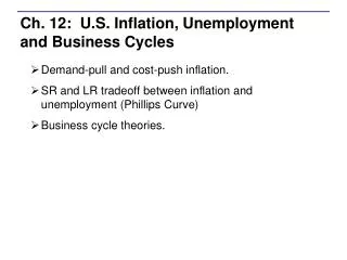
Eco 106 W8B Contrasting Views of Inflation and Unemployment Case-Fair Ch 14. Unemployment Types and Flows Classical and Keynesian views of the Labor Market The Phillips Curve Inflation expectations US supply and demand shocks Okun’s Law The Taylor Rule and the FAIR model.

E N D
Eco 106 W8BContrasting Views ofInflation and UnemploymentCase-Fair Ch 14 Unemployment Types and Flows Classical and Keynesian views of the Labor Market The Phillips Curve Inflation expectations US supply and demand shocks Okun’s Law The Taylor Rule and the FAIR model
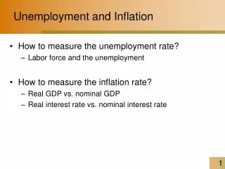
The Labor Market: Basic Concepts The labor force (LF) is the number of employed plus unemployed: LF = E + U unemployment rate The number of people unemployed as a percentage of the labor force. Unemployment rate = U/LF
The Labor Market: Basic Concepts frictional unemployment The portion of unemployment that is due to the normal working of the labor market; used to denote short-run job/skill matching problems. structural unemployment The portion of unemployment that is due to changes in the structure of the economy that result in a significant loss of jobs in certain industries. cyclical unemployment The increase in unemployment that occurs during recessions and depressions.
Ue Duration Most spells are short but at any moment in time the Unemployed population is dominated by longer term Unemployed. For example suppose: 2 mo. Spells, 60m spells for the year, 10m at any time 1 yr spells, 20m spells, 20m at any time Average spell= (60/80)2 mo+(20/80)12mo=4.5
Figure 3.15 Change in employment status in a typical month Change in employment status in a typical month The US labor market has huge “churn” relative to the net change in employment. Net Change in Employment here is -0.36, that is 1/5th of one percent of the Employed
Employment Situation • Has both Household and Establishment Data • Household survey has been showing more job growth. • Changes are small in comparison to totals • The Employment Situation from the BLS
Big Numbers 2.4 million jobs lost (reduction in employment) over 2008. 1.9m in last 4 months of year (post panic from Lehman Brothers collapse.) 2.6m long term unemployed (27 weeks or more). (Table A-12, Current Employment Situation, Friday Jan 9 2009)
2 sources of employment data household establishment
The Classical View of the Labor Market labor demand curve A graph that illustrates the amount of labor that firms want to employ at each given wage rate. labor supply curve A graph that illustrates the amount of labor that households want to supply at each given wage rate.
The Classical View of the Labor Market FIGURE 14.1 The Classical Labor Market Classical economists believe that the labor market always clears. If the demand for labor shifts from D0 to D1, the equilibrium wage will fall from W0 to W1. Anyone who wants a job at W1 will have one.
The Classical View of the Labor Market The Classical Labor Market and the Aggregate Supply Curve The classical idea that wages adjust to clear the labor market is consistent with the view that wages respond quickly to price changes. This means that the AS curve is vertical. When the AS curve is vertical, monetary and fiscal policy cannot affect the level of output and employment in the economy.
Sticky Wages vs Market Clearing W S With a perfectly functioning market an adverse supply shock will lower wages and employment. With “sticky wages” that shock would cause a greater fall in employment as well as unemployment rather than a falling real wage. D D’ N W S D D’ N
Keynesian vs Classical View of Ue K view: shocks to labor demand come from both the supply side (productivity and oil prices) and the demand side (C+I+G+X-IM). sticky wages cause labor demand shocks to become unemployment rather than lower wages. C view: shocks to labor demand come essentially from productivity shocks.
The Classical View of the Labor Market The Unemployment Rate and the Classical View The unemployment rate is not necessarily an accurate indicator of whether the labor market is working properly. The measured unemployment rate may sometimes seem high even though the labor market is working well.
Explaining the Existence of Unemployment Sticky Wages sticky wages The downward rigidity of wages as an explanation for the existence of unemployment. FIGURE 14.2 Sticky Wages If wages “stick” at W0 instead of falling to the new equilibrium wage of W* following a shift of demand from D0 to D1, the result will be unemployment equal to L0 - L1.
Explaining the Existence of Unemployment Sticky Wages Social, or Implicit, Contracts social, or implicit, contracts Unspoken agreements between workers and firms that firms will not cut wages. relative-wage explanation of unemployment An explanation for sticky wages (and therefore unemployment): If workers are concerned about their wages relative to other workers in other firms and industries, they may be unwilling to accept a wage cut unless they know that all other workers are receiving similar cuts.
Explaining the Existence of Unemployment Sticky Wages Explicit Contracts explicit contracts Employment contracts that stipulate workers’ wages, usually for a period of 1 to 3 years. cost-of-living adjustments (COLAs) Contract provisions that tie wages to changes in the cost of living. The greater the inflation rate, the more wages are raised.
Explaining the Existence of Unemployment Sticky Wages Explicit Contracts Graduate School Applications in Recessions Graduate School Offers Relief During Economic Recession Oklahoma Daily (U. Oklahoma)
Explaining the Existence of Unemployment Efficiency Wage Theory efficiency wage theory An explanation for unemployment that holds that the productivity of workers increases with the wage rate. If this is so, firms may have an incentive to pay wages above the market-clearing rate.
Explaining the Existence of Unemployment Imperfect Information Firms may not have enough information at their disposal to know what the market-clearing wage is. In this case, firms are said to have imperfect information. If firms have imperfect or incomplete information, they may set wages wrong—wages that do not clear the labor market.
Explaining the Existence of Unemployment Minimum Wage Laws minimum wage laws Laws that set a floor for wage rates—that is, a minimum hourly rate for any kind of labor. An Open Question The aggregate labor market is very complicated, and there are no simple answers to why there is unemployment.
The Short-Run Relationship Betweenthe Unemployment Rate and Inflation In the short run, the unemployment rate (U) and aggregate output (income) (Y) are negatively related. FIGURE 14.3 The Aggregate Supply Curve The AS curve shows a positive relationship between the price level (P) and aggregate output (income) (Y).
The Short-Run Relationship Betweenthe Unemployment Rate and Inflation This curve shows a negative relationship between the price level (P) and the unemployment rate (U). As the unemployment rate declines in response to the economy’s moving closer and closer to capacity output, the price level rises more and more.
The Short-Run Relationship Betweenthe Unemployment Rate and Inflation inflation rate The percentage change in the price level. Phillips Curve A curve showing the relationship between the inflation rate and the unemployment rate.
The Short-Run Relationship Betweenthe Unemployment Rate and Inflation The Phillips Curve shows the relationship between the inflation rate and the unemployment rate.
The Short-Run Relationship Betweenthe Unemployment Rate and Inflation The Phillips Curve: A Historical Perspective During the 1960s, there seemed to be an obvious trade-off between inflation and unemployment. Policy debates during the period revolved around this apparent trade-off.
In the 1950’s 60’s and 70’s the two political parties were associated with different preferences regarding where the economy should operate on the Phillips curve Inflation Unemployment
The Short-Run Relationship Betweenthe Unemployment Rate and Inflation The Phillips Curve: A Historical Perspective From the 1970s on, it became clear that the relationship between unemployment and inflation was anything but simple.
The Short-Run Relationship Betweenthe Unemployment Rate and Inflation Aggregate Supply and Aggregate Demand Analysis and the Phillips Curve FIGURE 14.8 Changes in the Price Level and Aggregate Output Depend on Shifts in Both Aggregate Demand and Aggregate Supply
In the 1960’s the Phillips curve was viewed as a stable trade off Between inflation and unemployment. It is a menu, we thought. Just pick which point you like best. Able and Bernanke Figure 12.01 The Phillips curve and the U.S. economy during the 1960s
Demand Pull then Supply Push • Pi is the inflation rate. • There is a special point on any Phillips curve that shows the natural rate of unemployment and the expected rate of inflation. Unemployment rate
Demand Pull then Supply Push Late 60’s • In the late 60’ the economy stayed above expected inflation and so inflation expectations rose. Phillips Curve of 1970’s Phillips Curve of 1960’s Unemployment rate
The Short-Run Relationship Betweenthe Unemployment Rate and Inflation Expectations and the Phillips Curve Expectations are self-fulfilling. This means that wage inflation is affected by expectations of future price inflation. Price expectations that affect wage contracts eventually affect prices themselves. Inflationary expectations shift the Phillips Curve up and to the right.
US 70’s Late 1960’s Demand Pull Inflation
The Short-Run Relationship Betweenthe Unemployment Rate and Inflation Aggregate Supply and Aggregate Demand Analysis and the Phillips Curve The Role of Import Prices FIGURE 14.9 The Price of Imports, 1960 I–2007 IV
US 80’s 2nd Oil Shock 1979 Oil Shock and After
Why Can’t I Draw? 79 inf 73 Early 80’s End 60’s Late 90’s Ue
The Short-Run Relationship Betweenthe Unemployment Rate and Inflation Is There a Short-Run Trade-Off between Inflation and Unemployment? There is a short-run trade-off between inflation and unemployment, but other factors besides unemployment affect inflation. Policy involves more than simply choosing a point along a nice smooth curve.
The Long-Run Aggregate Supply Curve, Potential Output, and the Natural Rate of Unemployment FIGURE 14.10 The Long-Run Phillips Curve: The Natural Rate of Unemployment If the AS curve is vertical in the long run, so is the Phillips Curve. In the long run, the Phillips Curve corresponds to the natural rate of unemployment—that is, the unemployment rate that is consistent with the notion of a fixed long-run output at potential output. U* is the natural rate of unemployment.
The Long-Run Aggregate Supply Curve, Potential Output, and the Natural Rate of Unemployment natural rate of unemployment The unemployment that occurs as a normal part of the functioning of the economy. Sometimes taken as the sum of frictional unemployment and structural unemployment.
The Long-Run Aggregate Supply Curve, Potential Output, and the Natural Rate of Unemployment The Nonaccelerating Inflation Rate of Unemployment (NAIRU) To the left of the NAIRU, the price level is accelerating (positive changes in the inflation rate); to the right of the NAIRU, the price level is decelerating (negative changes in the inflation rate). Only at the NAIRU is inflation constant.
4 Okun’s Law • Only mentioned in passing by Fair, useful for your paper!
Okun’s law How does unemployment vary with output. How does unemployment vary in response to the Growth rate of output? What is the potential growth rate of the economy?