Download
1 / 106
1.06k likes | 1.32k Vues
SWISS Score. Nice Graphical Introduction:. SWISS Score. Toy Examples (2-d): Which are “More Clustered?”. SWISS Score. Toy Examples (2-d): Which are “More Clustered?”. SWISS Score. Avg. Pairwise SWISS – Toy Examples. Hiearchical Clustering. Aggregate or Split, to get Dendogram

E N D
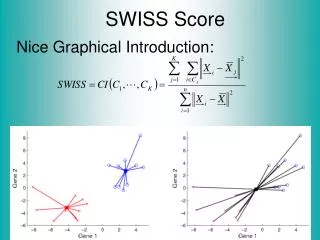
SWISS Score Nice Graphical Introduction:
SWISS Score Toy Examples (2-d): Which are “More Clustered?”
SWISS Score Toy Examples (2-d): Which are “More Clustered?”
SWISS Score Avg. Pairwise SWISS – Toy Examples
Hiearchical Clustering Aggregate or Split, to get Dendogram Thanks to US EPA: water.epa.gov
SigClust • Statistical Significance of Clusters • in HDLSS Data • When is a cluster “really there”? Liu et al (2007), Huang et al (2014)
DiProPerm Hypothesis Test Suggested Approach: • Find a DIrection (separating classes) • PROject the data (reduces to 1 dim) • PERMute (class labels, to assess significance, with recomputed direction)
DiProPerm Hypothesis Test Finds Significant Difference Despite Weak Visual Impression Thanks to Josh Cates
DiProPerm Hypothesis Test Also Compare: Developmentally Delayed No Significant Difference But Strong Visual Impression Thanks to Josh Cates
DiProPerm Hypothesis Test Two Examples Which Is “More Distinct”? Visually Better Separation? Thanks to Katie Hoadley
DiProPerm Hypothesis Test Two Examples Which Is “More Distinct”? Stronger Statistical Significance! Thanks to Katie Hoadley
DiProPerm Hypothesis Test Value of DiProPerm: • Visual Impression is Easily Misleading (onto HDLSS projections, e.g. Maximal Data Piling) • Really Need to Assess Significance • DiProPerm used routinely (even for variable selection)
Interesting Statistical Problem For HDLSS data: • When clusters seem to appear • E.g. found by clustering method • How do we know they are really there? • Question asked by Neil Hayes • Define appropriate statistical significance? • Can we calculate it?
Simple Gaussian Example Results: • Random relabelling T-stat is not significant • But extreme T-stat is strongly significant • This comes from clustering operation • Conclude sub-populations are different • Now see that: Not the same as clusters really there • Need a new approach to study clusters
StatisticalSignificance of Clusters Basis of SigClust Approach: • What defines: A Single Cluster? • A Gaussian distribution (Sarle & Kou 1993) • So define SigClust test based on: • 2-means cluster index (measure) as statistic • Gaussian null distribution • Currently compute by simulation • Possible to do this analytically???
SigClustStatistic – 2-Means Cluster Index Measure of non-Gaussianity: • 2-means Cluster Index • Familiar Criterion from k-means Clustering • Within Class Sum of Squared Distances to Class Means • Prefer to divide (normalize) by Overall Sum of Squared Distances to Mean • Puts on scale of proportions
SigClustGaussian null distribut’n Which Gaussian (for null)? Standard (sphered) normal? • No, not realistic • Rejection not strong evidence for clustering • Could also get that from a-spherical Gaussian • Need Gaussian more like data: • Need Full model • Challenge: Parameter Estimation • Recall HDLSS Context
SigClust Gaussian null distribut’n Estimated Mean, (of Gaussian dist’n)? • 1st Key Idea: Can ignore this • By appealing to shift invariance of CI • When Data are (rigidly) shifted • CI remains the same • So enough to simulate with mean 0 • Other uses of invariance ideas?
SigClust Gaussian null distribut’n 2nd Key Idea: Mod Out Rotations • Replace full Cov. by diagonal matrix • As done in PCA eigen-analysis • But then “not like data”??? • OK, since k-means clustering (i.e. CI) is rotation invariant (assuming e.g. Euclidean Distance)
SigClust Gaussian null distribut’n 2nd Key Idea: Mod Out Rotations • Only need to estimate diagonal matrix • But still have HDLSS problems? • E.g. Perou 500 data: Dimension Sample Size • Still need to estimate param’s
SigClust Gaussian null distribut’n 3rd Key Idea: Factor Analysis Model
SigClust Gaussian null distribut’n 3rd Key Idea: Factor Analysis Model • Model Covariance as: Biology + Noise Where • is “fairly low dimensional” • is estimated from background noise
SigClust Gaussian null distribut’n Estimation of Background Noise :
SigClust Gaussian null distribut’n Estimation of Background Noise : • Reasonable model (for each gene): Expression = Signal + Noise
SigClust Gaussian null distribut’n Estimation of Background Noise : • Reasonable model (for each gene): Expression = Signal + Noise • “noise” is roughly Gaussian • “noise” terms essentially independent (across genes)
SigClust Gaussian null distribut’n Estimation of Background Noise : Model OK, since data come from light intensities at colored spots
SigClust Gaussian null distribut’n Estimation of Background Noise : • For all expression values (as numbers) (Each Entry of dxn Data matrix)
SigClust Gaussian null distribut’n Estimation of Background Noise : • For all expression values (as numbers) • Use robust estimate of scale • Median Absolute Deviation (MAD) (from the median)
SigClust Gaussian null distribut’n Estimation of Background Noise : • For all expression values (as numbers) • Use robust estimate of scale • Median Absolute Deviation (MAD) (from the median)
SigClust Gaussian null distribut’n Estimation of Background Noise : • For all expression values (as numbers) • Use robust estimate of scale • Median Absolute Deviation (MAD) (from the median) • Rescale to put on same scale as s. d.:
SigClust Estimation of Background Noise n = 533, d = 9456
SigClust Estimation of Background Noise Hope: Most Entries are “Pure Noise, (Gaussian)”
SigClust Estimation of Background Noise Hope: Most Entries are “Pure Noise, (Gaussian)” A Few (<< ¼) Are Biological Signal – Outliers
SigClust Estimation of Background Noise Hope: Most Entries are “Pure Noise, (Gaussian)” A Few (<< ¼) Are Biological Signal – Outliers How to Check?
Q-Q plots An aside: Fitting probability distributions to data
Q-Q plots An aside: Fitting probability distributions to data • Does Gaussian distribution “fit”??? • If not, why not?
Q-Q plots An aside: Fitting probability distributions to data • Does Gaussian distribution “fit”??? • If not, why not? • Fit in some part of the distribution? (e.g. in the middle only?)
Q-Q plots Approaches to: Fitting probability distributions to data • Histograms • Kernel Density Estimates
Q-Q plots Approaches to: Fitting probability distributions to data • Histograms • Kernel Density Estimates Drawbacks: often not best view (for determining goodness of fit)
Q-Q plots Consider Testbed of 4 Toy Examples: • non-Gaussian! • non-Gaussian(?) • Gaussian • Gaussian? (Will use these names several times)
Q-Q plots Simple Toy Example, non-Gaussian!
Q-Q plots Simple Toy Example, non-Gaussian(?)
Q-Q plots Simple Toy Example, Gaussian
Q-Q plots Simple Toy Example, Gaussian?
Q-Q plots Notes: • Bimodal see non-Gaussian with histo • Other cases: hard to see • Conclude: Histogram poor at assessing Gauss’ity
Q-Q plots Standard approach to checking Gaussianity • QQ – plots Background: Graphical Goodness of Fit Fisher (1983)
Q-Q plots Background: Graphical Goodness of Fit Basis: Cumulative Distribution Function (CDF)
Q-Q plots Background: Graphical Goodness of Fit Basis: Cumulative Distribution Function (CDF) Probability quantile notation: for "probability” and "quantile"
Q-Q plots Probability quantile notation: for "probability” and "quantile“ Thus is called the quantile function
Q-Q plots Two types of CDF: • Theoretical