Download
1 / 49
540 likes | 840 Vues
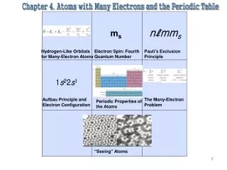
Chapter 4. Atoms with Many Electrons and the Periodic Table. nℓmm s. m s. Hydrogen-Like Orbitals for Many-Electron Atoms. Electron Spin: Fourth Quantum Number. Pauli’s Exclusion Principle. 1 s 2 2 s 1. Aufbau Principle and Electron Configuration. The Many-Electron Problem.

E N D
Chapter 4. Atoms with Many Electrons and the Periodic Table nℓmms ms Hydrogen-Like Orbitals for Many-Electron Atoms Electron Spin: Fourth Quantum Number Pauli’s Exclusion Principle 1s22s1 Aufbau Principle and Electron Configuration The Many-Electron Problem Periodic Properties of the Atoms “Seeing” Atoms
Chapter 4. Atoms with Many Electrons and the Periodic Table 4.1 Hydrogen-like Orbitals for Many-Electron Atoms He-atom (z = 2)Fig. 4.1 2 electrons labeled 1, 2 , coordinates r1≡ (r1,θ1,Ф1); r2≡ (r2,θ2,Ф2) Hamiltonian operator, Ĥ (electron-electron repulsion) r12 ≡┃r1 – r2┃ r12 → inter-electron distance Interparticle distance in He Screening of an electron by another
r1≡ (r1,θ1,Ф1) interelectron distance r12 ≡┃r1 – r2┃ r2≡ (r2,θ2,Ф2) Repulsion between electrons: This new cross-term makes the Schrodinger equation impossible to solve exactly and causes the Bohr model to fail for He and other atoms Interparticle distance in He Screening of an electron by another
Correlated Motion · r12– no fixed relation to the electron-nucleus distance due to the mobility of both electrons. · The electrons try to avoid each other to minimize the potential energy of the system. Ψ(r1,r2) → large amplitude whenr1and r2 are small but r12 is large. Interacting term to the wave function · Hartree and Slater (early 1930s) e2/r12 → neglecting this term, the total potential energy was cancelled by ca. 25%. · all electrons → were treated as independent, meaning that we neglect the repulsion term. Then : one electron orbital
Screening Effect ·|ψa(r1)|2→screens the nuclear charge to a small extent from electron 2, and vice versa · Effect → is incorporated into the orbitals by replacing the actual nuclear charge Z = 2 by an “effective” nuclear charge Zeff. [ex. Zeff (He) = 1.6875] (4.3) Orbital Approximation vs. Observation (Spectroscopy) 1st IE 2nd IE Total (eV) Orbital approx. -77.46 (Eq.4.3) UV spectrum -24.59 -54.40 -78.99 Absolute error = 1.53 eV (1.9%)
For the ground state of He, 1s2 occupancy 1s orbital 1s orbital
How about Z=3 (Li atom)? 1s3 ? => In this case Li’s IE would be even higher than He’s. However, in reality, the IE of Li is only 5.39 eV. Compare this with 24.59 eV for the IE of He. It turns out to be 1s22s1 instead of 1s3. Why? This is related with another dimension, an intrinsic property of the electron called spin.
4.2 Electron Spin: Evidence for a Fourth Quantum Number ms Electron Spin ·Na D-line transition ( a closely spaced doublet) 3s 3p vibrationrotation of the electron around the Na+ ion core ·circulating charge → generates a magnetic field · Uhlenbeck and Goudsmit (1925) ascribes an intrinsic angular momentum or spin s of the electron and accompanying magnetism due to the charged electron’s spinning on its axis. spin quantum number s → 1/2 projection of it → +1/2 or -1/2
Fig.4.2 Uhlenbeck andGoudsmit’s explanation of Na D Doublet The rotation of a charged particle around the nucleus and the spin itself → generate two magnets. If these two magnets are in the same direction (m =+1, ms=+1/2), → they repel each other. (V is higher) If they are opposed (m =+1, ms=-1/2), → they attract. (V is lower) 3s → 3p transition Y 00 (3s) → no vibration 3p orbital of Na atom → exerts doublet.
Discovery of Electron Spins One day earlier Ehrenfest had written to Lorentz to make an appointment for the coming Monday to discuss a "very witty idea" of two of his graduate students. When Lorentz pointed out that the idea of a spinning electron would be incompatible with classical electrodynamics, Uhlenbeck asked Ehrenfest not to submit the paper. Ehrenfest replied that he had already sent off their note, and he added: "You are both young enough to be able to afford a stupidity!" Ehrenfest's encouraging response to his students ideas contrasted sharply with that of Wolfgang Pauli. As it turned out, Ralph Kronig, a young Columbia University PhD who had spent two years studying in Europe, had come up with the idea of electron spin several months before Uhlenbeck and Goudsmit. He had put it before Pauli for his reactions, who had ridiculed it, saying that "it is indeed very clever but of course has nothing to do with reality". Kronig did not publish his ideas on spin. No wonder that Uhlenbeck would later refer to the "luck and privilege to be students of Paul Ehrenfest".
Stern-Gerlach Experiment: Experimental evidence for the existence of electron spin Stern and Gerlach (1926) Ground stateNa atoms → were passed through a strong inhomogeneous magnetic field. · All spin magnetisms in inner orbitals → cancelled, except an electron in 3s orbital. ·Y (θ,Ф)(3s) → no rotation ·Theintrinsic magnetismof the 3s electron → only possibleto respond to the external field. · 3s electrons → line up with their north poles either along or against the main north pole of the magnet. The lack of a “straight-through” beam with the magnet → clear evidence of two-valued electron’s magnetism.
Dirac (1928) · Using the Schrödinger’s idea and Einstein’s (1905) special theory of relativity → 4 coupled Schrödinger-like equations (Dirac Eq) · Dirac equations → 4th quantum number, ms (Electrons are required to have spin: a law of nature, NOT a postulate) ·Diracpredicted → antimatter (antiparticle: negative energy) Dirac Equation of spin -1/2 particles (relativistic modification of the Schrödinger wave equation) Dirac’s Relativistic Electron
Paul A. M. Dirac 1902-1984 (England) 1928, Prediction of Positron 1932, Observation of positron 1930, “Principles of Quantum Mechanics” 1933, Nobel Prize (w/ Schrödinger) Founder of Quantum Electrodynamics
4.3 Pauli’s Exclusion Principle W. Pauli (1925) No two electrons in a given atom → can have the same set of four quantum numbers { n, ℓ, m, ms} ex.He (Z = 2) 1s2: (100+½) and (100-½) Li (Z = 3) → 1s22s1 NOT 1s3 !! n =1(100+½) (100-½), n =2 (200+½) Each orbital (n, l, m) can hold at most 2 electrons with ms +½ or -½ Magnetic implications ! Wolfgang Pauli 1900-1958 (Austria) 1925, Proposal of the exclusion theory 1945, Nobel Prize
4.4 Aufbau Principle and Electron Configurations of the Elements Aufbau principle (Building–up principle): a rule for electronic configuration. The ground-state electron configuration of an atom → add the electrons (Z in number) one by one into the lowest energy orbitals available. Energies of Orbitals: Screening Li (Z = 3) ·1s22s1vs. 1s22p1← Two orbitals (2s and 2p both) are degenerate states · 2s or 2p orbital → experiences the screening of the nucleus by 1s2 electrons · Since 2s has inner “hump” which is closer to the nucleus, a 2s electron sees a larger effective nuclear charge. 1s-2s gap: 70 eV in Li 2s-2p gap: 1.8 eV in Li
Second Period Elements Li – Ne (z = 3 – 10) 1s2 part → invariant for the entire period, core electrons, and play little role in the structure and reactions. 2s, 2p parts → form the periphery of the second row atoms. endow the elements with their chemical power, valence electrons Shell: 2n2 Due to spin Sub-shell: 2(2l+1)
Hund’s Rule Degenerate orbitals → always fills with single electrons before any of them are doubly occupied. Unpaired electrons Paired electrons
Reading Configurations from the Periodic Table Electron Configurations ·Two most important effects: (i) Screening effect shell (n) → splits into n ℓ subshells (n=2 into 2s and 2p, n=3 into 3s, 3p, 3d, n=4 into 4s, 4p, 4d, 4f, n=5 into 5s, 5pf, 5d, 5f, 5g) (ii) Energy drawing effect drawing together in energy of successive n shells [The gap between E(n=2) and E(n=3) is smaller than the gap between E(n=1) and E(n=2)] Because of these effects, a high-ℓ orbital of a given n may be higher in energy than a low-ℓ orbital of the n + 1 (4s<3d). ·n = 3 period capacity of electrons in n-shell: 2n2 = 18 → 8 observed, 10 missing electrons in ℓ- subshell: 2(2ℓ + 1) = 2(2x2 + 1) = 10 → filled in 3d Because of the screening of n =1and n =2 shells 3d level → higher than 4s
·n = 4 period Fig.4.6 The “long form” of the periodic table 4s2, 3d10, 4p6 ·n = 5 5s2, 4d10, 5p6 ·n = 6 6s2, 4f14, 5d10, 6p6 ← ns, (n -2)f, (n -1)d, np ·n = 7 ←starts out like the sixth period, but is incomplete as yet.
Fig.4.7 Splitting and interleaving of Orbital energies due to screening
Anomalous Configurations Exceptions to the Aufbau principle due to e-e pairing E * For Cu, 4s14d10 instead of 4s24d9
4.5 Periodic Properties of the Atoms of the Elements Orbital energy ← as a function of Z and n Fig.4.8 Orbital energies as a function of Z
Ionization Energy First IE The energy to remove the most weakly bound electron or the electron from the highest occupied (valence) atomic orbital (HOAO ). ex. B (Z = 5) 8.30 (1st IE), 25.15(2nd), 37.93(3rd), 259.4(4th), 340.2 eV(5th) Be(9.32) > B(8.30 eV) Be → 2s subshell is filled and no more valence electron B → 2p1more effectively screened by 2s2, the increase in Zeffis insufficient to bridge 2s-2p energy gap.
N (14.53) > O(13.62) N → 2p subshells are half-filled with 3 unpaired electrons O → One of 2p-subshells is paired. The repulsion between these electrons is not offset by the increase in Zeff. IE (i ) Increase from left to right in the periodic table. (ii) Decrease from top to bottom. (iii) Increase from lower left to upper right. Transition elements, Lanthanides, and Actinides (i) The electrons are filling inner shells, while the losing electrons are from the outer s orbitals. (ii) The Zeffis relatively constant across a d- or f-series till the d-subshell or f-subshell is fully filled.
The last IE (the “Zth”) corresponds to creation of a bare nucleus and can be computed accurately from the Bohr formula. For Hydrogen Atom, the IE is rigorously equal to the negative of the ground state orbital energy: IE1= -E1 = +13.6 eV For bigger atoms (for example carbon) this relationship is only approximate; the remaining electrons relax a bit due to the loss of electron-electron repulsion. IE < -EHOAO C+: 1s22s22p1 C+: 1s22s22p1 energy relaxing -EHOAO IE C: 1s22s22p2 C: 1s22s22p2
For transition elements, the last electron fills inner shell, but the electrons that are lost in ionization come from the outer s orbitals instead. For example for Ti, Ti+:[Ar]4s23d1 Ti+:[Ar]4s13d2 Energy Ti:[Ar]3d4 Ti:[Ar]4s23d2
Periodic table of IE (eV) Overall trend in IE
Electron Affinity Electron affinity (EA) The energy required to remove the least tightly bound electron to leave a neutral atom. EA < IE EA → no Coulomb attraction between A (neutral atom) and e-. A- should have room to share the subshell by the new electron, which increases e-…e- repulsion. EA << -EHOAO with an extra electron
Fig.4.11 EA vs. Z and Periodic Table of EAs (eV) Choppier than Fig.4.9 because of the requirement of the vacancy of the subshell for the new electrons.
Electron affinity (i) The elements with filled shell or subshell have no electron affinity. (ii) EA has the same trends as for IE, increasing from lower left to upper right. (iii) EA of 3rd period > that of 2nd period. It is because of the leading role of electron repulsion in determining the stability of the negative ion. Since 3n orbitals are larger than 2n orbitals, the distance among the electrons increase. → Size effect
Atomic Radius rnℓ -the radius of peak probability in the radial distribution function Fig.4.12 Atomic radius vs. Z Periodic table of atomic radii (Å)
Atomic Radius (i) The radius does not show the irregularities due to subshell structure. (ii) The anomalously high IEs for the sixth period (5d ) transition metals → correlate with the small atomic radii. The filling of the 4f subshell prior to 5d causes an increase in Zeffand correspondingly shrinks the valence orbitals. → Lanthanide Contraction ·n = 4: 4s2, 3d10, 4p6 ·n = 5: 5s2, 4d10, 5p6 ·n = 6: 6s2, 4f14, 5d10, 6p6
Ionic Configurations and Isoelectronic Sequences N3- O2- F- Na+ Mg2+ Al3+ electronic configuration → appeared to be same 1s22s22p6 → isoelectronic ions radii decrease due to the steadily increasing nuclear charge N3- Al3+
Fig. 4.13 Atomic (shaded spheres) and ionic (dashed circles) in pictorial form
4.6 Computers in Chemistry: The Many-Electron Problem SCF( Self-consistent-field) (Hartree, 1928-1936) computer calculations Hamiltonian operator Ĥ for an atom with N electrons (N = Z ) (4.8) rij → interelectron distance (only i < j terms) ex. Na (Z = 11) Hamiltonian 77 terms: Electron-electron repulsion 55 terms; Wave function 33 dimensional
Total wave function Hartree assumed (cf. Eq. 4.2) orbital product: (4.9) the repulsion term (4.10) (i ) ψα→ the orbital occupied by the electron j and integrated over the volume ← neglected the correlated motion. The integral was taken every possible position of j. (ii ) The repulsion term now depends only on the i. (independent particle approximation with ‘mean-field’) (iii) Substituting Eqs. (4.9), (4.10) into (4.8), the equation breaks up into N one-electron equations. (iv) Using the iteration technique, the guess work can be remedied.
This approximation took several months to produce results for Na in 1930’s It becomes almost trivial for atoms and small molecules now on computers This SCF method and the extensions developed by ‘quantum chemists’ can supplement experiment for many molecules Quantum chemical calculations are now become one of the routine tools for chemists
ComputationalQuantum Chemistry can be used to obtain energies and orbitals for many different chemical systems
4.7 “Seeing” Atoms Electron diffraction(L. Bartell and L. Brockway, 1953) · By passing 40 KeV electrons through Ar atomic beam, very short de Broglie wavelength, shorter than x-ray, was enabled to see the details of the electron cloud. · The image of the scattered electrons → depicted the electron shells of Ar clearly. Radial electron distribution for Ar good agreement between the experiment and the orbital model (3 maxima: n = 1, 2, 3)
Scanning Tunneling Microscopy (STM) (G. Binning and H. Rohrer, 1982 IBM, Nobel Prize in 1991) · A sharply pointed electrode tip, is located within a few angstroms of a solid surface of a metal or a semiconductor. · Applying a small voltage between the tip and the surface, it causes electrons to “tunnel” out of the surface into the tip. Department of Chemistry, KAIST
Firg.4.15 (a) STM image of Si-crystal, Si-Si; (b) A higher tip bias, Si-Si bond · The tip is directly above the metal and its height is controlled by feedback control to keep constant current. · Varying the bias of the tip: 1) Low-bias → surface map of the atom 2) Higher bias → electrons located “between” the atoms, “bonding” electrons. The resulting current is a map of atoms on the surface
Chemical Capabilities Fig.4.16 a) pure Si-surface b) treated with NH3 to form Si-H bonds Seeing is Believing ! 百聞不如一見
Atomic force microscopy (AFM) · Tip is very close to the surface and dragged over it. · Deflections of the tip arm → are detected by laser reflection. · AFM can be used for any types of surface either the metal or the non-metal. Fig.4.18 AFM images of the surface of graphite (left) and a sodium chloride crystal (right)
Scanning Probe Microscopy (SPM) · SPM → comprises all the techniques. · They are all enabled by the piezoelectric effect, utilizing a piezoelectric crystal to probe. SPM images of amorphous carbon film grown at 800℃ Department of Chemistry, KAIST