Download

1 / 7
70 likes | 91 Vues
CBitss technologies are the best institute for Advanced Excel Training in Chandigarh. Functioning skilled person connected to accounts, to learn Advanced Microsoft Excel, Access, VBA, Macro, and advanced commands and techniques to get familiar with Excel

E N D
Advance Excel training in Chandigarh
INTRODUCTION Advanced Excel is a comprehensive Presentation that provides a good insight into the latest and advanced features available in Microsoft Excel 2013. It has plenty of screenshots that explain how to use a particular feature, in a step-by-step manner.
Change in Charts Group The Charts Group on the Ribbon in MS Excel 2013 looks as follows − You can observe that − • The subgroups are clubbed together. • A new option ‘Recommended Charts’ is added. Let us create a chart. Follow the steps given below. Step 1 − Select the data for which you want to create a chart. Step 2 − Click on the Insert Column Chart icon as shown below. When you click on the Insert Column chart, types of 2-D Column Charts, and 3-D Column Charts are displayed. You can also see the option of More Column Charts. Step 3 − If you are sure of which chart you have to use, you can choose a Chart and proceed. If you find that the one you pick is not working well for your data, the new Recommended Charts command on the Insert tab helps you to create a chart quickly that is just right for your data.
Chart Recommendations Let us see the options available under this heading. (use another word for heading) Step 1 − Select the Data from the worksheet. Step 2 − Click on Recommended Charts. Step 3 − As you browse through the Recommended Charts, you will see the preview on the right side. Step 4 − If you find the chart you like, click on it. Step 5 − Click on the OK button. If you do not see a chart you like, click on All Charts to see all the available chart types. Step 6 − The chart will be displayed in your worksheet. Step 7 − Give a Title to the chart.
Click on the Chart. Three Buttons appear next to the upper-right corner of the chart. They are − • Chart Elements • Chart Styles and Colors, and • Chart Filters You can use these buttons − • To add chart elements like axis titles or data labels • To customize the look of the chart, or • To change the data that’s shown in the chart Fine Tune Charts Quickly
The readers of this presentation are expected to have a good prior understanding of the basic features available in Microsoft Excel. Next presentation to discuss more advance excel features. Know abou training process. Call us- 09988741983 Address: SCO: 24-25, Piccadilly Road, Sub. City Center, Sector 34A, Sector 23, Chandigarh, 160022 Website: http://advancedexceltraininginchandigarh.blogspot.in