Paleo-intensity (PI)
Paleo-intensity (PI). Geomagnetic field: full vector field So far: declination & inclination Up next: intensity. Intensity Earth ’ s magnetic field. Unit: Tesla (T) 1 T = 1 N / (Am) ~ 20 to 60 μT (NL: 48.9 μT) Understanding geodynamo action


Paleo-intensity (PI)
E N D
Presentation Transcript
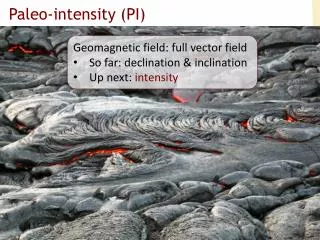
Paleo-intensity (PI) • Geomagnetic field: full vector field • So far: declination & inclination • Up next: intensity
Intensity Earth’s magnetic field • Unit: Tesla (T) 1 T = 1 N / (Am) • ~ 20 to 60 μT (NL: 48.9 μT) • Understanding geodynamo action • Intensity dropped 12% since recording began: onset of a field reversal? • Interactions of inner & outer core, core & mantle: improving dynamo models • Atmospheric interaction: variable field shielding in relation to residence times and deposition of cosmogenic isotopes (radiometric dating!)
Enhanced solar activity Quebec blackout: 6 million people without power for 9 hrs. March 1989: solar storm
Intensity Earth’s magnetic field + + _ + _
Observations from space Hulot et al., 2002: Intensity dipole field decreases through growth of `reversed flux patch’ in Southern Atlantic Ocean. If continued at present pace then field would reverse in ~1500 years or so.
PI in the “news” “The Observer” November 2002
And of course … • Movie • Websites: • www.the-end.com • www.ijstijd.com • www.goto2012.nl • Etc.
Paleo-intensity • Two `tastes’: • Absolute PI • Using `(p)TRMs’ (thermal: volcanics) • Spot-readings, dated • Relative PI • Using `DRMs’ (detrital: sediments) • Comparative in nature, time sequences
Absolute PI: working with (p)TRMs pTRMs are independent and additive Tauxe, 2005
Absolute PI – the principle Main assumption: TRM HTRM field Y < field A = field X < field Z Partially replacing the NRM with a pTRM due to a known field.
Absolute PI - different methods • Thellier style (Thellier, 1955) • Varying T in constant H • Using one specimen • Multi-specimen style (MSP) (Dekkers, 2006) • Varying H in constant T • Use more specimens
Thellier-style - “ARAI-plot” HNRM = - slope * Hlab
Multi-Specimen Style ( pTRM – NRM ) / NRM HNRM given by x-axis-intercept
So we’re all set ... ? Both methods work perfectly fine for thermally stable SD grains, but… SD grains are very rare in nature! Some problems: • Chemical alteration • Alteration of the magnetic state • Unblocking T ? = blocking T • Magnetic treatment history (`tails’) `Multi-domain behaviour’
What can we do to avoid these problems ? • Determine the maximum T to use in the experiment, before the onset of alteration • Test our results for MD-behaviour • Success rate of Thellier: 0 – 30% • Success rate of MSP: ? (too few data so far)
Tests for chemical alteration Tests to determine the maximum T to use: Curie-balance measurements Susceptibility-vs-T experiments Day-plots before and after heating
Chemical alteration tackled … Alteration T is now known, but… Changes in magnetic state and bias due to multiple heating steps are still there Two main problems left: Multi-domain behaviour (magnetic treatment) Changes in the way magnetization is acquired
Magnetic Force Microscopy De Groot, Bakelaar, Dekkers, 2011/2012 Pristine Heated in 40 mT
MD behaviour in Thellier-style experiments “Sagging” Dunlop et al., 2005 JGR
How important is this “sagging”? Slope ≈ -2.7 Class exercise: Take two different slopes and calculate the corresponding PI. Hlab= 40 uT 2.7 x 40 = 108 uT 0.6 x 40 = 24 uT Dunlop et al., 2005 JGR Slope ≈ -0.6
Many Thellier-style protocols Per temperature step: Zero-field, In-field Per temperature step: In-field, Zero field Alternate these two: “IZZI” protocol Incorporate pTRM and pTRM tail checks Microwave excitation instead of thermal heating Include low-temperature demagnetization “Quasi-perpendicular” method Sample material: Plagioclase single crystals Sample material: Submarine basaltic glass
MSP examples (Dekkers & Boehnel, 2006) Expected field: 50.6 uT pTRM acquisition temperature 400°C Measured field (uT): ( ± 1 st.dev.) PT: 48.4 ± 2.23 Placer: 47.6 ± 2.22 ST: 52.7 ± 2.06 ST demagnetized at 200°C before & after pTRM acq.
MSP examples: Maui, Hawaii Lava flow ages: 200 – 8200 years
MSP examples: Maui, Hawaii 120 C 560 C 560 C 120 C 560 C 560 C
MSP examples: Maui, Hawaii pTRMacquisitiontemperature below alteration
Absolute PI: Hawaii Hawaii data compiled by Pressling et al., 2006
Another MSP example: Mt. Etna 1971 1983 IGRF field: 44 uT
MSP behavior Class exercise: What happens with the samples (in terms of acquisition) if an underestimate is observed? Would that behavior imply an over- or an underestimate in a Thellier-style experiment?
MSP behavior (pTRM-NRM)/NRM (expected) < (pTRM-NRM)/NRM (altered) pTRM(expected)< pTRM(altered) Samples must have acquired MOREpTRM to yield anUNDERestimate
Consequences for Thellier Samples that acquire MORE pTRM than expected, flatten the slope in a Thellier-style experiment, also yielding anUNDERestimate
Check for magnetic alteration EGU 2011: De Groot, Dekkers, Mullender ARM-acquisition test: AF-demagnetization in the presence of a DC-field (compares with pTRM: thermal-demagnetization in the presence of a DC-field)
ARM-experiments: results ARM-pristine > ARM-heated overestimated PI +50% ARM-pristine < ARM-heated underestimated PI -30% ARM-pristine ≈ ARM-heated ≈ correct PI
Wrap-up absolute PI Laborious experiments Low success rates But… We’re getting there More checks… eventually maybe a correction ?
Relative paleointensity • Detrital Remanent Magnetization (DRM) • Sediments records • Ocean drill cores • Compares intensities through continuous sections (thus through continuous time) Main assumption: MDRM HDRM
Normalization of DRM • Relative PIs need to be normalised because of differences in: • Magnetic activity • Concentration of magnetic particles • Mass & shape of samples • Sedimentation rates • … • Normalized to ARM, IRM or susceptibility (c) Think of relative PIs as the percentage of the potential magnetisation of a sample that was magnetised by Earth’s field at time of sedimentation
Normalizers: χ, ARM, or IRM c = magneticsusceptibility ARM = Anhysteretic Remanent Magnetization IRM = Isothermal Remanent Magnetization <100mT
Relative PI: considerations DRM: true detrital origin, high stability NRM: demagnetised (AF / TH) Concentration variation must be ‘small’ Magnetic mineralogy and grain sizemust be ~constant No coherence with bulk rock magnetic properties Spatially and temporally coherent, many records Independent time scale required
Variability in magnetic properties ODP core Atlantic Ocean Normalize Oligocene and Eocene portions separately Tauxe, 2005 chapter 8