Submodularity for Distributed Sensing Problems
This presentation explores the concept of submodularity and its applications in distributed sensing problems. Key topics include non-myopic maximization of information gain, path planning, and robust maximization/minimization strategies. Submodularity is defined and illustrated through examples, including set functions and sensor coverage. The greedy algorithm for approximate maximization is discussed, showcasing its effectiveness and guarantees. The limitations of existing algorithms are also highlighted, along with potential new techniques for optimizing sensor placements and path planning.


Submodularity for Distributed Sensing Problems
E N D
Presentation Transcript
Submodularity for Distributed Sensing Problems Zeyn Saigol IR Lab, School of Computer Science University of Birmingham 6th July 2010
Outline • What is submodularity? • Non-myopic maximisation of information gain • Path planning • Robust maximisation and minimisation • Summary * These slides are borrowed from Andreas Krause and Carlos Guestrin (see http://www.submodularity.org/) Submodularity
Set functions Y“Sick” Y“Sick” X1“Fever” X2“Rash” X2“Rash” X3“Male” F({X1,X2}) = 0.9 F({X2,X3}) = 0.5 • Submodularity in AI has been popularised by Andreas Krause and Carlos Guestrin • Finite set V = {1,2,…,n} • Function F: 2V R • Example: F(A) = IG(XA; Y) = H(Y) – H(Y | XA) = y,xA P(xA) [log P(y | xA) – log P(y)] Submodularity
Submodular set functions A B AB • Set function F on V is called submodular if For all A,B V: F(A)+F(B) F(AB)+F(AB) • Equivalent diminishing returns characterization: + + B A + S B Large improvement Submodularity: A + S Small improvement For AB, sB, F(A {s}) – F(A) F(B {s}) – F(B) Submodularity
Example problem: sensor coverage Place sensorsin building Possiblelocations V For A V: F(A) = “area covered by sensors placed at A” Node predicts values of positions with some radius Formally: W finite set, collection of n subsets SiW For A V={1,…,n} define F(A) = |iASi| Submodularity
Set coverage is submodular S’ A={S1,S2} S1 S2 S’ F(A{S’})-F(A) ≥ F(B{S’})-F(B) S1 S2 S3 S4 S’ B = {S1,S2,S3,S4} Submodularity
Approximate maximization Given: finite set V, monotonic submodular function F(A) Want: A* V such that NP-hard! Y“Sick” M Greedy algorithm: Start with A0 = {}; For i = 1 to k si := argmaxs F(Ai-1{s})-F(Ai-1) • Ai := Ai-1{si} X1“Fever” X2“Rash” X3“Male” 7 Submodularity
Guarantee on greedy algorithm ~63% Sidenote: Greedy algorithm gives 1/2 approximation for maximization over anymatroid C! [Fisher et al ’78] Theorem [Nemhauser et al ‘78] Given a monotonic submodular function F, F()=0, the greedy maximization algorithm returns Agreedy F(Agreedy) (1-1/e) max|A|k F(A) Submodularity
Example: Submodularity of info-gain Y1 Y2 Y3 X1 X2 X3 X4 Y1,…,Ym, X1, …, Xn discrete RVs F(A) = IG(Y; XA) = H(Y)-H(Y | XA) • F(A) is always monotonic • However, NOT always submodular Theorem [Krause & Guestrin UAI’ 05]If Xi are all conditionally independent given Y,then F(A) is submodular! Hence, greedy algorithm works! In fact, NO practical algorithm can do better than (1-1/e) approximation! 9 Submodularity
Information gain with cost • Instead of each sensor having the same measurement cost, variable cost C(X) for each node • Aim: max F(A) s.t. C(A) B where C(A)=XAC(X) • In this case, construct every possible 3-element subset of V, and run greedy algorithm on each • Greedy algorithm selects additional nodes X by maximising • Finally choose best set A • Maintains (1 − 1/e) approximation guarantee Submodularity
Path planning maxA F(A) or maxA miniFi(A) subject to • So far: |A| k • In practice, more complex constraints: Sensors need to communicate (form a routing tree) [Krause et al., IPSN 06] Locations need to be connected by paths[Chekuri & Pal, FOCS ’05][Singh et al, IJCAI ’07] Lake monitoring Building monitoring Submodularity
Informative path planning s4 Most informative locationsmight be far apart! 2 1 2 s1 1 s5 s2 1 s3 1 s10 1 s11 1 So far: max F(A) s.t. |A|k Robot needs to travelbetween selected locations Locations V nodes in a graph C(A) = cost of cheapest path connecting nodes A max F(A) s.t. C(A) B Submodularity
The pSPIEL Algorithm [K, Guestrin, Gupta, Kleinberg IPSN ‘06] C1 C2 S1 SB C4 C3 • pSPIEL: Efficient nonmyopic algorithm (padded Sensor Placements at Informative and cost-Effective Locations) Select starting and endinglocation s1and sB Decompose sensing region into small, well-separated clusters Solve cardinality constrained problem per cluster (greedy) Combine solutions using orienteering algorithm Smooth resulting path g2,2 g1,2 g1,1 g2,1 g1,3 g2,3 g4,3 g3,1 g3,3 g4,4 g4,1 g3,2 g3,4 g4,2 Submodularity
Limitations of pSPEIL • Requires locality property – far apart observations are independent • Adaptive algorithm [Singh, Krause, Kaiser IJCAI‘09] • Just re-plans on every timestep • Often this is near-optimal; if it isn’t, have to add an adaptivity gap term to the objective function U to encourage exploration Submodularity
Submodular optimisation spectrum • Maximization: A* = argmax F(A) • Sensor placement • Informative path planning • Active learning • … • Optimise for worst case: • Minimization: A* = argmin F(A) • Structure learning (A* = argmin I(XA; XVnA)) • Clustering • MAP inference in Markov Random Fields Submodularity
Summary Submodularity is useful! Submodularity