Fourier Transforms

1. Fourier Transforms

2. Background • While the Fourier series/transform is very important for representing a signal in the frequency domain, it is also important for calculating a system’s response (convolution). • A system’s transfer function is the Fourier transform of its impulse response • Fourier transform of a signal’s derivative is multiplication in the frequency domain: jwX(jw) • Convolution in the time domain is given by multiplication in the frequency domain (similar idea to log transformations)

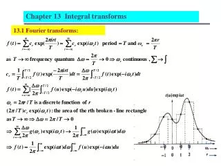
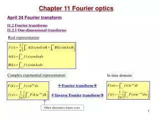
3. Fourier Series in exponential form Consider the Fourier series of the 2T periodic function: Due to the Euler formula It can be rewritten as With the decomposition coefficients calculated as: (1) (2)

4. Fourier transform The frequencies are and Therefore (1) and (2) are represented as Since, on one hand the function with period T has also the periods kT for any integer k, and on the other hand any non-periodic function can be considered as a function with infinite period, we can run the T to infinity, and obtain the Riemann sum with ∆w→∞, converging to the integral: (3) (4)

5. Fourier transform definition The integral (4) suggests the formal definition: The funciotn F(w) is called a Fourier Transform of function f(x) if: The function Is called an inverse Fourier transform of F(w). (5) (6)

6. Example 1 The Fourier transform of is The inverse Fourier transform is

7. Fourier Integral If f(x) and f’(x) are piecewise continuous in every finite interval, and f(x) is absolutely integrable on R, i.e. converges, then Remark: the above conditions are sufficient, but not necessary.

8. Properties of Fourier transform 1 Linearity: For any constants a, b the following equality holds: Proof is by substitution into (5). • Scaling: For any constant c, the following equality holds:

9. Properties of Fourier transform 2 • Time shifting: Proof: • Frequency shifting: Proof:

10. Properties of Fourier transform 3 • Symmetry: Proof: The inverse Fourier transform is therefore

11. Properties of Fourier transform 4 • Modulation: Proof: Using Euler formula, properties 1 (linearity) and 4 (frequency shifting):

12. Differentiation in time • Transform of derivatives Suppose that f(n) is piecewise continuous, and absolutely integrable on R. Then In particular and Proof: From the definition of F{f(n)(t)} via integrating by parts.

13. Example 2 The property of Fourier transform of derivatives can be used for solution of differential equations: Setting F{y(t)}=Y(w), we have

14. Example 2 Then Therefore

15. Frequency Differentiation In particular and Which can be proved from the definition of F{f(t)}.

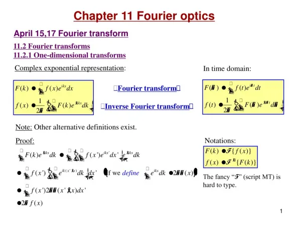
16. Fourier Transform • A CT signal x(t) and its frequency domain, Fourier transform signal, X(jw), are related by • This is denoted by: • For example: • Often you have tables for common Fourier transforms • The Fourier transform, X(jw), represents the frequency content of x(t). • It exists either when x(t)->0 as |t|->∞ or when x(t) is periodic (it generalizes the Fourier series) analysis synthesis

17. Linearity of the Fourier Transform • The Fourier transform is a linear function of x(t) • This follows directly from the definition of the Fourier transform (as the integral operator is linear) & it easily extends to an arbitrary number of signals • Like impulses/convolution, if we know the Fourier transform of simple signals, we can calculate the Fourier transform of more complex signals which are a linear combination of the simple signals

18. Fourier Transform of a Time Shifted Signal • We’ll show that a Fourier transform of a signal which has a simple time shift is: • i.e. the original Fourier transform but shifted in phase by –wt0 • Proof • Consider the Fourier transform synthesis equation: • but this is the synthesis equation for the Fourier transform • e-jw0tX(jw)

19. x1(t) t x2(t) t x(t) t Example: Linearity & Time Shift • Consider the signal (linear sum of two time shifted rectangular pulses) • where x1(t) is of width 1, x2(t) is of width 3, centred on zero (see figures) • Using the FT of a rectangular pulse L10S7 • Then using the linearity and time shift Fourier transform properties

20. Fourier Transform of a Derivative • By differentiating both sides of the Fourier transform synthesis equation with respect to t: • Therefore noting that this is the synthesis equation for the Fourier transform jwX(jw) • This is very important, because it replaces differentiation in the time domain with multiplication (by jw) in the frequency domain. • We can solve ODEs in the frequency domain using algebraic operations (see next slides)

21. Convolution in the Frequency Domain • We can easily solve ODEs in the frequency domain: • Therefore, to apply convolution in the frequency domain, we just have to multiply the two Fourier Transforms. • To solve for the differential/convolution equation using Fourier transforms: • Calculate Fourier transforms of x(t) and h(t): X(jw) by H(jw) • MultiplyH(jw) by X(jw) to obtain Y(jw) • Calculate the inverse Fourier transform of Y(jw) • H(jw) is the LTI system’s transfer function which is the Fourier transform of the impulse response, h(t). Very important in the remainder of the course (using Laplace transforms) • This result is proven in the appendix

22. Example 1: Solving a First Order ODE • Calculate the response of a CT LTI system with impulse response: • to the input signal: • Taking Fourier transforms of both signals: • gives the overall frequency response: • to convert this to the time domain, express as partial fractions: • Therefore, the CT system response is: assume ba

23. H(jw) -wc wc w h(t) 0 t Example 2: Design a Low Pass Filter • Consider an ideal low pass filter in frequency domain: • The filter’s impulse response is the inverse Fourier transform • which is an ideal low pass CT filter. However it is non-causal, so this cannot be manufactured exactly & the time-domain oscillations may be undesirable • We need to approximate this filter with a causal system such as 1st order LTI system impulse response {h(t), H(jw)}:

24. Convolution The convolution of two functions f(t) and g(t) is defined as: Theorem: Proof:

25. Appendix: Proof of Convolution Property • Taking Fourier transforms gives: • Interchanging the order of integration, we have • By the time shift property, the bracketed term is e-jwtH(jw), so

26. Summary • The Fourier transform is widely used for designing filters. You can design systems with reject high frequency noise and just retain the low frequency components. This is natural to describe in the frequency domain. • Important properties of the Fourier transform are: • 1. Linearity and time shifts • 2. Differentiation • 3. Convolution • Some operations are simplified in the frequency domain, but there are a number of signals for which the Fourier transform does not exist – this leads naturally onto Laplace transforms. Similar properties hold for Laplace transforms & the Laplace transform is widely used in engineering analysis.

27. Lecture 11: Exercises • Theory • Using linearity & time shift calculate the Fourier transform of • Use the FT derivative relationship (S7) and the Fourier series/transform expression for sin(w0t) (L10-S3) to evaluate the FT of cos(w0t). • Calculate the FTs of the systems’ impulse responses • a) b) • Calculate the system responses in Q3 when the following input signal is applied • Matlab/Simulink • Verify the answer to Q1 using the Fourier transform toolbox in Matlab • Verify Q3 and Q4 in Simulink • Simulate a first order system in Simulink and input a series of sinusoidal signals with different frequencies. How does the response depend on the input frequency (S12)?