Chapter 13: Chi-Square Procedures
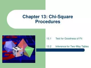
Chapter 13: Chi-Square Procedures. 13.1 Test for Goodness of Fit 13.2 Inference for Two-Way Tables. M&Ms Example. Sometimes we want to examine the distribution of proportions in a single population. As opposed to comparing distributions from two populations, as in Chapter 12.

Chapter 13: Chi-Square Procedures
E N D
Presentation Transcript
Chapter 13: Chi-Square Procedures 13.1 Test for Goodness of Fit 13.2 Inference for Two-Way Tables
M&Ms Example • Sometimes we want to examine the distribution of proportions in a single population. • As opposed to comparing distributions from two populations, as in Chapter 12. • Does the distribution of colors in your bags match up with expected values? • We can use a chi-square goodness of fit test. • Χ2 • We would not want to do multiple one-proportion z-tests. • Why?
Performing a X2 Test 1. H0: the color distribution of our M&Ms is as advertised: Pbrown=0.30, Pyellow=Pred=0.20, and Porange=Pgreen=Pblue=0.10 Ha: the color distribution of our M&Ms is not as advertised. • Conditions: • All individual expected counts are at least 1. • No more than 20% of expected counts are less than 5. • Chi-square statistic:
X2 Family of Distribution Curves • Used to assess the evidence against H0 represented in the value of X2. • The member of the family we choose is determined only by the degrees of freedom. • P-value is the probability of observing a value X2 at least as extreme as the one actually observed.
Performing a test with our calculators • Enter data: • L1: observed values (not percentages) • L2: expected values • L3: (L1-L2)2/L2 • LIST/MATH Sum (L3) • X2cdf(ans,1099, df)
Practice • Exercise 13.10, p. 743
More Practice • Exercise 13.4, p. 737
13.4 Follow-Up • So we reject the null, but so what? • What does this mean in the context of the problem? • Where did the differences occur?
Example 13.4, pp. 744-748 • Is there a difference between proportion of successes? • At left is a two-way table for use in studying this question. • Explanatory Variable: • Type of Treatment • Response Variable: • Proportion of no relapses
Example 13.4, pp. 744-748 • H0: p1=p2=p3 • Ha: at least one proportion is not equal to the others.
Example 13.4, pp. 744-748 • We need expected counts for each cell: • For our example, 2/3 relapsed (48/72). So, if Ho is true, then 24(2/3) of those taking Desipramine would relapse. • Write expected counts for each cell in your table at the bottom of page 747.
Chi-Square Test forHomogeneity of Populations • In this example, we are comparing the proportion of relapses in three populations: addicts who take desipramine, addicts who take lithium, and addicts who take a placebo. • Our question is this: Are the populations homogeneous in terms of the proportion of relapsed addicts? • We use a chi-square test for homogeneity of populations.
Conditions • All individual expected counts are at least one, and • No more than 20% of expected counts are less than 5.
Calculations for Example 13.4 Note: df=(#r-1)(#c-1)=(3-1)(2-1)=2
Full Analysis of Example 13.4 • See Example 13.7, p. 752
Practice • 13.14, pp. 748-749
Let’s begin with a practice problem … • 13.15, p. 749 + 13.17, p. 756
Two Settings for Chi-Square Testsfor Two-Way Tables • Yesterday we studied the problem of treatments for cocaine addicts. The cocaine addicts study is an experiment that assigned 24 addicts to each of three groups. Each group is a sample from a separate population corresponding to a separate treatment. • We used a chi-square test for homogeneity of populations. (H0: p1=p2=p3 vs. Ha: at least one not the same) • Today, we look at problems where subjects from a single sample are classified with respect to a categorical variable. • We will use a chi-square test of association/independence. • Notes: • See bottom paragraph, p. 763. • The analysis for today’s problem will be essentially identical to the analysis from yesterday.
Example • 13.9, 13.10, and 13.11, pp. 758-761 • Hypotheses: • H0: there is no relationship between smoking status and SES (two categorical variables). • Ha: there is a relationship between smoking status and SES.
Expected Counts and Conditions • All expected counts are at least 1, no more than 20% less than 5.
Practice Problem • 13.20, p. 762 • Make a bar graph to show the data graphically before beginning your calculations for the chi-square test.
Practice • 13.32, p. 770 • Chapter 13 Test on Tuesday.

